Determination of Some Trace Elements in Marine Sediment using ICP-MS and XRF (A Comparative Study)

Introduction

Some of the sources of trace elements as pollutants are, vehicle emission, agricultural, industrial and shipping activities [1], [2]. [3]. The health risk of trace elements in aquatic environment and subsequent uptake in the food chain by aquatic organisms and humans, can results in morphological abnormalities and genetic alteration of cells. In addition, trace elements can affect enzymatic and hormonal activities [1]. It is important to evaluate metal content in sediments because under certain conditions, sediment can act as a sink as well as a source of metals. Moreover, the amount of a given metal that can be released from contaminated sediment depends critically on the metal species [4].

Both X-ray fluorescence (XRF) and inductively coupled plasma-mass spectrometry (ICP-MS) are widely used as multi-elemental analytical techniques to study metals in water and sediment [5]. ICP-MS is a very rapid, multielement and accurate analytical technique with very low detection limits for most elements (ppb). For XRF it is a fast multi elemental technique with detection limit of few ppm. [6].

The aim of this study is to compare the applicability of ICP-MS and XRF techniques for the determination of trace elements in marine sediment samples. The comparison will define the possible element concentrations levels determined by the techniques and assist in identifying the best technique for analyzing specific elements in marine sediments.

Material and methods

Samples Collection

Sediment samples were collected from coasts of Sabah and Sarawak states, located in East Malaysia, where oil and gas exploration and production activities are the major cause of marine pollution.  The area lay between 1º45.93´ to 7 º24.68´ N latitude and 109 º49.20´ to 119 º 03.78´ E Longitude.  22 sites, as shown in Figure 1, were selected along the coasts where a total of 75 samples were collected at different distances from the coast (between 0.7-113 m) Another 12 surface sediment samples (depth 1 meter) were collected at the coast of Taman Negara Bako Sarawak (six samples) and from the coast of Taman Negara Pulau Talang Sarawak (another six samples). Both areas, as shown in Figure 2, are considered as pristine as both were the national parks and used as control samples.

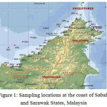Figure 1: Sampling locations at the coast of Sabah and Sarawak States, Malaysia Click here to View figure

 

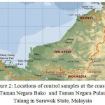Figure 2: Locations of control samples at the coast of Taman Negara Bako  and Taman Negara Pulau Talang in Sarawak State, Malaysia Click here to View figure

 

All sediment samples were collected using sediment grab and stored in polyethylene containers.

All samples were dried in an oven at 50ºC and homogenized by powdering in an agate mortar. Before analysis, the powder samples were heated at 50º C until constant weight was established. The moisture content of the samples was determined prior to analysis.

Samples Preparation for ICP-MS

Method of Digestion

Microwave digestion program as reported by Delphin et al[7] and Sandroni [8] was used. 0.5 g of each dry sample was accurately weighed and added with 6 ml of 17 M HNO₃, 2 ml of 8.8M H₂O₂ and 2 ml of 0.02 M HF. The samples were digested in a microwave oven (MARS 5 from CEM) using program as of Perez-Santana [9]: 5min at 300W, 20min at 540W, 5min at 60 W. For quality control purposes, standard reference materials (SRM) (soil -7), marine sediment (PACS-2) and stream sediment (SL-1)) were treated as above. Blank samples were also prepared for each set by adding the digestion acids mixture used above without adding the sample.

Sample Analysis using ICP-MS

All samples, standards and blanks solutions as prepared above were analyzed using PE SCIEX ELAN 6000 ICP-MS system.

Samples Preparation for XRF

1.00 g of each dry sample was accurately weighed and pressed using manual hydrolic pressing machine (20 tons). The pellet diameter was 40mm.  Standard reference material SRM (soil-7) was treated as above. Blank or control samples were also prepared for each set.

The prepared pallets of samples, standards and blanks were then analyzed using BRUKER S8 TIGER XRF system.

Statistical Analysis

Two statistical analysis methods for the analysis of the data namely the two sided t-test and the paired t-test, were applied in this work:

Two Sided T-tests

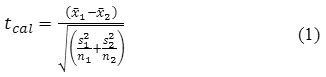
The two sided t-test is applied to check if methods under comparison provide same results, by comparing their means and standard deviations. For the comparison of the means without assuming equal variances equation (1) is used [10], [11]:

Where

is the mean of the first method,

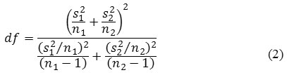
is the mean of the second method, s₁ and s₂are the respective variances, and n₁ and n₂are the respective number of measurements. The test is performed by calculating the t value from equation (1) and comparing it with t_a/2  of the tabulated t-distribution at α level of significance and with degrees of freedom as in equation (2) [12].

When the  t_cal > t _a/2 , it can be concluded that the difference between the means obtained by the two methods is statistically significant. If the t_cal > t _a/2 , it can be concluded that there is no significant difference between the two methods.

Paired T- Test

In this test equal numbers of measurements must be done in both methods, since each sample is measured in both methods. Then the mean of the differences between the two methods was calculated for each of the samples,

and also the standard deviation of the differences, s. The statistic t is calculated by the equation (3)

Where n is the number of pairs (samples measured by both methods) and the degrees of freedom, df is equal to (n-1) [10].

Results and discussion

ICP-MS Measurements

Quality control of the obtained data was performed through the analysis of the certified reference materials (CRMs).Tables 1-3 show the analytical and the certified values, the error, and recovery for the studied elements with the respect to the CRMs.

Table 1: Comparison of the ICP-MS results obtained in this work with the certified values for the CRM of soil-7.

Elements	Value found (ppm)	Certified value (ppm)	Recovery %	Error
Al	33407.00	47000.00	71.08	0.29
V	*	66.00	*	*
Cr	51.40	60.00	85.67	0.14
Mn	635.50	631.00	100.71	0.01
Fe	19550.00	25700.00	76.07	0.24
Co	10.01	8.90	112.43	0.12
Ni	30.39	26.00	116.89	0.17
Cu	19.38	11.00	176.22	0.76
Zn	188.46	104.00	181.22	0.812
As	15.46	13.40	115.35	0.15
Se	0.38	0.40	94.00	0.06
Cd	2.78	1.30	213.86	1.14
Pb	69.09	60.00	115.15	0.15

Table 2: Comparison of the ICP-MS results obtained in this work with the certified values for the CRM of PACS-2.

Elements	Value found(ppm)	Certified value(ppm)	Recovery %	Error
Al	5922.00	6620.00	89.46	0.11
V	140.05	133.00	105.30	0.05
Cr	87.59	90.70	96.57	0.03
Mn	446.64	440.00	101.51	0.02
Fe	35656.00	4090.00	871.78	7.72
Co	11.47	11.50	99.70	0.003
Ni	42.42	39.50	107.39	0.07
Cu	346.39	310.00	111.74	0.12
Zn	717.17	364.00	197.02	0.97
As	30.60	26.20	116.80	0.17
Se	1.09	0.92	118.91	0.19
Cd	3.59	2.11	169.96	0.70
Pb	223.17	183.00	121.95	0.22

 

Table 3: Comparison of the ICP-MS results obtained in this work with the certified values for the CRM of SL-1.

Elements	Value found(ppm)	Certified value(ppm)	Recovery  %	Error
V	187.40	170.00	110.24	0.10
Cr	90.36	104.00	86.89	0.13
Mn	3115.48	3460.00	90.04	0.10
Fe	48160.00	67400.00	71.45	0.29
Co	19.84	19.80	100.20	0.001
Ni	53.40	44.90	118.93	0.19
Cu	32.18	30.00	107.26	0.07
Zn	792.73	223.00	355.49	2.55
As	29.07	27.60	105.31	0.05
Se	4.11	2.85	144.39	0.44
Cd	0.39	0.26	151.08	0.51
Pb	57.58	37.70	152.74	0.53

 

From Table1 it can clearly be observed that for soil-7  Mn, Se, Cr, show good recovery and low error, and to some extend Ni, Co, As, and Pb.  For PACS-2 in Table 2 Al, Mn, Cr, Co, V, Ni, Cu and to some extend Se, As, and Pb show acceptable results.

For  Sl-1 (Table 3) V, Cr, Mn, Co, Cu, As, and to some extend Ni show acceptable results.

From these observations (Table 1, 2 and 3) it can be concluded that in this study the ICP/MS give acceptable results for all elements under study except for Cd, Fe, and Zn. For Cd this may be due to isobaric interference because all isotopes of Cd may interfere with various isobaric ions and/or oxide or hydroxide ions of other trace elements. If the concentrations of these interference elements are larger than the Cd concentration in soils or sediments, it could lead to significantly erroneous results [13]. For Fe, usually there is polyatomic interference as reported by (May) [14] especially for the isotope Fe ⁵⁶ (abundance 91%) and the concentration of Fe calculated using the other isotopes of the element which their abundance is very low. For Zn the high results appear in the three CRMs may be due to its high first ionization potentials (9.4 V) which may make it more sensitive to ‘spatial effects’ within the plasma [15].

To compare between the concentrations of the elements in the sediment samples and control samples using ICP-MS the two sided t-test is applied. The comparison is carried out between the samples from the depth A and the control samples, and the results are listed in Table 4.

Table 4: Comparison of the elements concentration between samples and control samples using ICP-MS.

Element	Samples		Control Samples		t (cal)	df
	Average (ppm)	SD	Average(ppm)	SD
As	17.30	11.50	36.43	51.83	-1.262	12
Cd	0.90	1.90	0.24	0.23	1.608	22
Co	12.10	7.10	5.12	0.56	4.585	21
Cr	71.00	67.90	43.06	20.67	1.784	27
Cu	34.30	40.20	9.69	4.07	2.845	22
Fe	26119.70	12103.20	9049.82	2707.41	6.331	25
Mn	495.00	249.00	343.37	56.23	2.731	25
Ni	51.20	46.90	11.83	2.91	3.924	21
Pb	49.80	41.60	18.78	4.02	3.468	22
Se	3.40	1.80	3.26	3.22	0.139	15
V	125.90	66.00	46.56	33.22	4.659	32
Zn	311.00	133.70	157.70	65.60	4.480	32

 

From Table 4 and from the table of values for the two-sided t-distribution all the elements concentrations show significant differences between the samples and the control samples except for As, Cd, Cr and Se. This result gives indication that all elements may have anthropogenic sources except As, Cd, Cr and Se since the control samples were collected from area supposed to be free from anthropogenic input.

Figure 3 shows the concentration of elements under study in the three depths using ICP-MS.

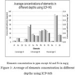Figure 3: Average of elements concentration in different depths using ICP-MS   Click here to View figure

 

From Figure 3 it’s clear that no significant variation in elements concentrations in the three depths, which implies that no significant anthropogenic input over the years at the study area.

XRF Measurements

Quality control for the obtained data was carried out using standard reference material (CRM) of soil-7. Table 5 shows the analytical and the certified values, the error, and recovery for the studied elements with the respect to the CRM.

Table 5: Comparison of the XRF results obtained in this work with the certified values for the CRM of soil-7.

Elements	Value found(ppm)	Certified value(ppm)	Recovery %	Error
As	24.00	13.40	179.10	0.79
Cd	0.30	1.30	23.08	0.77
Co	8.60	8.90	96.63	0.03
Cr	49.80	60. 00	83.00	0.17
Cu	22.60	11.00	205.45	1.06
Fe	25657.40	25700.00	99.83	0.002
Mn	498.20	631.00	78.95	0.21
Ni	33.40	26.00	128.46	0.29
Pb	33.10	60.00	55.17	0.45
Se	2.70	0.40	675.00	5.75
V	67.40	66.00	102.12	0.02
Zn	108.90	104.00	104.71	0.05

 

From Table 5 it can be clearly seen that the elements which show acceptable results are: Cr, Co, Fe, V, Zn, and to some extend Mn. This may be due to the detection limit of the XRF which is in limit of few ppm [16].

To compare between the concentrations of the elements in the sediment samples and control samples using XRF the two sided t-test is also applied. The comparison is carried out between the samples from the depth A and the control samples which are surface samples, and the results are listed in Table 6.

Table 6: Comparison of the elements concentration between samples and control samples using XRF.

Element	Samples		Control Samples		t (cal)	df
	Average (ppm)	SD	Average (ppm)	SD
As	1.30	25.10	1.86	25.27	-0.28	17
Cd	0.20	0.30	0.01	0.29	0.23	21
Co	1.80	13.60	1.06	8.59	10.20	32
Cr	22.70	80.80	3.92	52.98	5.60	23
Cu	2.30	28.30	0.65	25.29	5.74	27
Fe	10805.10	44474.00	6576.78	20.21	14.89	31
Mn	107.80	442.50	74.39	346.62	3.05	30
Ni	16.90	51.10	1.44	33.53	4.84	22
Pb	1.70	34.50	2.86	34.66	-0.18	15
Se	0.20	3.30	0.09	3.30	0.10	31
V	14.70	100.10	10.15	63.00	8.65	30
Zn	8.80	115.80	7.12	82.02	12.14	27

 

From Table 6 and from the table of values for the two-sided t-distribution all the elements concentrations show that there are significant differences between the samples and the control samples except for As, Cd, Pb and Se. This result and the result from table 4 give indication that all elements may have anthropogenic sources except As, Cd, and Se.

Fig.4 shows the concentration of elements under study in the three depths using XRF.

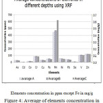Figure 4: Average of elements concentration in different depths using XRF Click here to View figure

 

From Figure 4 it’s clear that no significant variation in elements concentrations in the three depths- except Mn which show higher concentration in the third depth (avarage C).

Comparison Between XRF and ICP-MS Results

To compare between the ICP-MS and XRF used in this work paired t –test was applied. The results are shown in table 7.

Table 7: Comparison of XRF and ICP/MS by mean of paired t-test

Element	Mean difference   (µg /g)	S.D.of  mean difference (µg/g)	Calculated t
As	10.10	9.50	9.18
Cd	-1.00	6.00	-1.50
Co	1.50	10.30	1.24
Cr	19.30	53.60	3.11
Cu	-2.20	38.60	-0.49
Fe	20968.30	12693.00	14.31
Mn	72.10	379.70	1.65
Ni	0.90	38.70	0.21
Pb	-2.50	27.80	-0.79
Se	-0.00	2.10	-0.04
V	-9.10	70.50	-1.12
Zn	-158.60	152.90	-8.98

Theoretical t: p=95%  2.021, p=98% 2.423, p=99% 2.704.

 

As shown in Table 7, for 95%,  98% and 99% confident levels, Cd, Co, Cu, Mn, Ni, Pb, Se and V did not give significant differences, while As, Cr, Fe and Zn  give significant differences at all confident levels. From this test it can be concluded that the two techniques agree for most of the elements under study accept for As, Cr, Fe and Zn.

Conclusion

In view of the results obtained by the two techniques, we can look at two aspects. In terms of sample preparations, the XRF has advantage over ICP/MS. This is because ICP/MS not only require the use of strong acids, but also the longer digestion time. In addition ICP/MS is also a destructive technique. However, in terms of the range of elements that can be detected, ICP/MS has advantage over XRF since it has lower detection limit for most elements. The results from this study clearly indicates that the two detection techniques agree with each other on Cd, Co, Cu, Mn, Ni, Pb, Se and V results and did not agree on As, Cr, Fe and Zn.

Acknowledgement

The authors would like to thank the Universiti Kebangsaan Malaysia and Malaysian Nuclear Agency for supporting this work.

References

1. Bubb, J. M. and J. N. Lester, The impact of heavy metals on lowland rivers and the implications for man and the environment, Science of The Total Environment (1991), 100(0), 207-233.
2. Forstner, U., G. T. W. Wittmann, Metal pollution in the aquatic environment, Goldberg. Berlin;  Springer-Verlag (1979).
3. Idris, A. M., M. A. H. Eltayeb, Assessment of heavy metals pollution in Sudanese harbours along the Red Sea Coast,  Microchemical Journal, (2007),  87, 104-112.
4. Marqu´es, M. J., A. Salvador, Trace element determination in sediments: a comparative study between neutron activation analysis NAA/ and inductively coupled plasma-mass spectrometry ICP-MS/,  Microchemical Journal, (2000), 65: 177-187.
5. Smirnova, E. V., I. N. Fedorova, Determination of rare earth elements in black shales by inductively coupled plasma mass spectrometry, Spectrochimica Acta Part B: Atomic Spectroscopy, (2003), 58(2): 329-340.
6. Boyle, J. F., Rapid elemental analysis of sediment samples by isotope source XRF, Journal of Paleolimnology, (2000),  23(2): 213-221.
7. Delphine, N.-M., M.-R. Maria-Paz, New application of microwave digestion-inductively coupled plasma-mass spectrometry for multi-element analysis in komatiites, Analytica Chimica Acta, (2008), 628(2): 133-142.
8. Sandroni, V. and C. M. M. Smith, Microwave digestion of sludge, soil and sediment samples for metal analysis by inductively coupled plasma-atomic emission spectrometry, Analytica Chimica Acta,  (2002), 468(2): 335-344.
9. Perez-Santana, S., M. Pomares Alfonso, Total and partial digestion of sediments for the evaluation of trace element environmental pollution, Chemosphere, (2007), 66(8): 1545-1553.
10. Alfassi, Z. B., Z. Boger, Statistical treatment of analytical data, Blackwell Science, (2005).
11. Urdan, T. C., Statistics In Plain English, Mahwah, New Jersey, Lawrence Erlbaum Associates, Inc, (2005).
12. Davenport, J. M. and J. T. Webster,  Metrica, (1975).
13. Guo, W., Shenghong, Direct Determination of Trace Cadmium in Environmental Samples By Dynamic Reaction Cell Inductively Coupled Plasma Mass Spectrometry,  Chemosphere,  (2010) 81: 1463-1468.
14. May, T. W. and R. H. Wiedmeyer A Table Of Polyatomic Interferences In ICP-MS,  Atomic Spectroscopy, (1998), 19: 150-155.
15. Campbell, M. J. and A. To¨rve´nyi, Non-Spectroscopic Suppression Of zinc In ICP-MS In A Candidate Biological Reference Material (IAEA 392 Algae), J. Anal. At. Spectrom, (1999), 14: 1313-1316.
16. Moros, J., A. Gredill, Partial Least Squares X-Ray Fluorescence Determination of Trace Elements In Sediments From The Estuary of Nerbioi-Ibaizabal River, Talanta 82 (2010) 1254–1260.

---

This work is licensed under a Creative Commons Attribution 4.0 International License.