Kinetics of Biogas Production from Goat Dung and Pawpaw Seed

Introduction

Energy is an essential commodity in the world. In the past and present times, Nigeria has relied on the hydrostatic power plants for electricity generation¹ and fossil fuel for transportation. However, Nigeria’s energy grid is experiencing some crises due to lack of development. This problem is coupled with the fact that burning fossil fuel emits a lot of greenhouse gas (e.g. Carbon dioxide- CO₂), which causes environmental degradation and global warming. With such prevalent problems, there is need to consider alternative sources of energy as we seek to improve our energy supply. The key to making a more reliable energy sector is to find and use a renewable energy resource, rather than simply relying on the country’s non-renewable resources².

Biogas is generated when anaerobic microbes feed on carbohydrates and fats (without oxygen), producing CH₄ and CO₂ as waste products^{3, 4}. These microbes feed off fats, carbohydrates and proteins, and then through a complex chain of reactions generates biogas consisting mainly of methane (55-60%) and CO₂ (35-40%) along with traces of other gases such as H₂S (0-2%), H₂ (0-1%), N₂ (0-2%), O₂ (0-2%), water vapour, siloxanes, depending on the waste matter decomposed^{3, 5-8}. The constituents other than methane are contaminants and have various effects on the application of biogas or the environment. These negative impacts range from lowering its calorific value, corrosion of equipment and piping system, emitting SO₂ and NOx on combustion⁹.

Biogas can be used in several ways, either as raw or upgraded. It can be an alternative to fossil fuel.¹⁰In its raw state, biogas is utilized in the production of heat and electricity, while upgraded biogas is used as vehicle fuel, in which liquid fuels such as petrol and diesel are replaced⁵.It serves as green gas when introduced into the natural gas grids^{3, 11}. In addition, biogas is used to produce energy in Combined Heat and Power (CHP) units³. Indeed, if these inexpensive but essential wastes from plants and animals are properly harnessed, biogas technology could become a sustainable way to meet the future energy demands of rural households, especially those in developing countries.

For biogas to fulfill its potential as limitless and versatile source of sustainable energy, most of the contaminants present in it must be removed; and anaerobic digestion must be optimized with appropriate models that can be used in control theory¹². The process of removing CO₂ from the biogas to improve its energy content with the end product being bio-methane is known as biogas upgrading^{13, 14}.

To adequately harness the potentials of biogas technology in meeting present and future energy needs, it may not be enough to just produce biogas. There is need to assess the potentials of different biomasses, operational conditions and models, which could be useful in predictive mode for optimal production for mass utilization. This study is therefore, aimed at evaluating and assessing the quantity and quality of biogas generated from goat dung and pawpaw. The suitability of using selected anaerobic digestion models in predicting biogas production was also evaluated.

Materials and Methods

Material collection and preparation for anaerobic digestion

Pawpaw seeds used for this study were collected from ripe pawpaw (Carica papaya) fruits. The goat dung was collected from various goat sellers, while the cow dung used as inoculums was collected from fresh cow excreta. Both samples used for the mono-digestion were sun dried for several days to lower their moisture contents. After which they were ground into powder in order to increase their surface area and make them have fine particle sizes. Slurries of each of the samples were made by mixing 1000 g of each powdered sample with 3500 mL of water. This constitutes 22% total solid (TS) to maintain satisfactory stability¹⁵.One hundred gram (100 g) of fresh moist cow dung was added to each of the slurries as inoculums to boost the microbial counts of the samples. Fresh cow dung was chosen as the inoculums because it has been reported to contain all the vital groups of microbial consortium needed for anaerobic digestion process¹⁶.The slurry for co-digestion was also prepared in the same way, except that the co-digested substrate contained 1:1 mole ratio of a mixture of pawpaw seed and goat dung.

Digester set-up

The experiment was done at the Environmental Laboratory of Landmark University, Omu – Aran, Kwara State, Nigeria; using a five-liter automated twin anaerobic digester. The digester is an all-glass apparatus, housed in a glass water bath, whose temperature is automatically regulated by a computer system. The digester is also connected to a water displacement system to determine the volume of gas produced. Figures 1 and 2 show the digestion apparatus and the flow diagram of the digester set-up respectively.

Figure 1: Picture of the twin anaerobic digesters Click here to View figure

Figure 2: Digester Set–up for Production and Measurement of Biogas. Click here to View figure

Anaerobic digestion (AD)

The digestion of the slurry was carried out batch by batch and monitored for 24 days. 4000 mL of each of the slurries was packed into the digester and corked. The digester temperature was set at 35 ^OC. The slurry was stirred daily by the in-built stirrer of the digester. Stirring prevents caking of the slurry and also aids uniform temperature and bacteria distribution.¹⁷.

Measurement of the biogas produced

The biogas produced was measured every 24 hours to determine its production rate as shown in figure 2. This was done by checking the fall in the level of water in the graduated cylinder. The volume of biogas formed for each day is proportional to the amount of water expelled.^{18, 19}

Determination of volatile solid (VS)

Available organic matter for the action of bacteria during digestion constitutes volatile solid²⁰. This solid would burn off when subjected to a furnace temperature of about 550 ^OC.

The total solid residue was heated in a muffle furnace at 600 ^OC for 2 hours, after which it was cooled in a desiccator and weighed. The volatile solid was calculated using equation (1).

W_T = weight of dried residue from total solid

A = weight of residue after further heating at 600^OC

g = Initial sample weight

Determination of biochemical oxygen demand (BOD)

The dissolved oxygen meter (Mw 600 by Milwaukee) was first calibrated using a standard solution. Serial dilutions were done on the sample, and then initial dissolved oxygen (DO_i) reading was taken. The same sample was kept in the laboratory incubator (DNP-9052 by SANFA) for five days, after which, the final dissolved oxygen (DO_f) was measured. The BOD after five days is the difference between DO_i and DO_f.

Determination of chemical oxygen demand (COD)

The test tube heater was turned on and set to 150 ^OC, while the safety screen was positioned. The test tube was vigorously agitated to suspend all sediment. 2 mL of the sample slurry was introduced into the test tube with the aid of the pipette. The test tube was then covered and inverted slowly in order to allow mixture of the contents. A blank reagent was prepared similarly using 2 mL of deionized water in another test tube. Both tubes were placed in the heater and digested for 2 hours. The tubes were cooled and their photometric readings taken and recorded in mg/L.

Kinetic models for simulation of daily biogas production rate

Biogas production rates of goat dung, pawpaw seed and the mixture of both substrates were simulated using linear and polynomial plots on Microsoft Excel.

Linear regression equation

The linear equation of the biogas production rate for the ascending and descending limb is expressed by equation (2) below²¹.It is assumed that biogas production rate will increase linearly with increase in time and after reaching a maximum point, it would decrease linearly to zero with increase in time.

Y = a + bT (2)

y = biogas production rate in mL/day.

T = time in days for digestion.

a (mL/day) is a constant obtained from y-intercept of the graph of y vs T.

b (mL/day) is a constant obtained from the slope of the graph of y vs T.

For the ascending limb, the slope, b, is positive and it is negative for the descending limb.

Polynomial Regression Equation

The polynomial plot of the ascending and descending limb is represented by equation (3). Here, it is assumed that biogas production rate shows a polynomial increase in time and after reaching the peak, it will decrease in the same vein to zero with further increase in time.

y = aT² + bT + c                                               (3)

y is the biogas production rate (mL/day)

T is the retention time in days

a, b and c are regression constants.

Polynomial regression equation seems to be very reliable in predicting biogas production in anaerobic digestion of animal wastes^{22, 23}.

Empirical models for simulation of the cumulative biogas production

The evaluation of anaerobic digestion was carried out by fitting the experimental data into modified Gompertz and modified Logistic models.

Modified Gompertz Model

Gompertz function is presented in equation (4)

G_t = A × exp [ -exp (b – ct)]                            (4)

Where, G_t is Gompertz cumulative gas yield per time.

A is biogas production potential (mg/TS)

b and c are constants of the Gompertz model

t is cumulative time for biogas production in days²⁴.

The modified Gompertz equation is shown in equation (5)

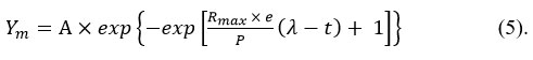
Y_m is cummulative biogas yield (mL) attime ( t )

R_max is maximum biogas production rate (mL/day).

t is retention time (days)

A is biogas production potential (mL)

e is mathematical constant; ^{24, 25}.

Equation (5) can be used to analyze biogas production. The P, R_max and λ, cannot be used for predictive purposes because they are limited to particular experimental conditions²⁶.

Modified Logistic Model

Equation (6) is an expression of the Logistic model.

L_t = A × [1 + exp (b – ct)] ^-1           (6)

Where, L_t is Logistic cumulative gas yield per time.

A is biogas production potential (m/g-TS)

b and c are constants of the Logistic model

t is cumulative time for biogas production in days²⁴.

The modified logistic function is shown in equation (7)  is modified and re-written thus:

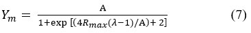
A is maximum production potential of biogas (mL)

R_max is maximum production rate of biogas(mL/day)

t is retention time in days

λ is lag phase/delay time in days.²⁴

The data from the three experiments were fitted into equations (5) and (7) using non-linear regression analysis with solver tool in Microsoft Excel 2007. The equations were used to determine biogas production potential (A), maximum production rate ( R_max ) and duration of the lag phase ( λ) . The predicted biogas yields from the non-linear regression analysis were plotted against the retention time and the experimental yields. The correlation coefficient (R²) was calculated using the regression data analysis tool in MS Excel, 2007. R² was obtained to examine the goodness of fit of the models to the experimental data. A confidence interval of 95% was chosen for the goodness of fit for the predicted data.R², visual inspection of the curve and experimental values must be taken into account to determine the suitability of the prediction models.

One-way analysis of variance (ANOVA) was performed using Microsoft Excel 2007 to determine whether there is significant difference between the experimental data and the predicted data for the biogas yield each of substrate. A confidence interval of 0.05 was chosen, hence, the difference was considered significant if the probability (p-value) was less than 0.05.

Results and Discussion

The physical and chemical properties of samples in this study are shown on table 1. The pH values of the substrates ranged from 7.12 to 7.46, this is presented in figure 3. This pH range is suitable for optimal performance of anaerobic digestion processes^{23, 27}.

Table 1: Physicochemical properties of the slurries before and after digestion.

Parameter	Goat Dung (GTD)		Pawpaw Seed (PPS)		Mixture
	Before	After	Before	After	Before	After
Ph	7.21	7.18	7.12	7.24	7.46	7.60
BOD5 (mg/L)	160	146	194	180	306	284
COD (mg/L)	490	312	480	346	512	286
TS (%)	15.10	11.70	16.30	12.80	20.60	14.40
VS (%)	84	66	86	72	82.80	64.40
TN(mg/L)	3.2	2.7	2.6	2.34	2.8	2.0
TC(mg/L)	28.3	22.0	32.3	28.6	43.2	38.6

 

Figure 3: Effect of anaerobic digestion on the pH of the slurries. Click here to View figure

The pH of goat dung after digestion dropped from 7.21 to 7.18, while that of pawpaw seed and the mixture increased from 7.12 to 7.24 and 7.46 to 7.60 respectively. The increase in pH for the latter could be attributed to the accumulation of ammonia²⁷, while the slight decrease in pH of goat dung slurry could be attributable to build-up of fatty acids and amino acid within the digester^{28, 29}. The pH values of the slurries after digestion indicate that they can be applied to soil, as fertilizers without adversely affecting the soil pH

There was a decrease in BOD, COD, TS and VS for goat dung, pawpaw seed and the mixture after the 24 days digestion period. Figure 4 shows the percentage decrease in the values of the aforementioned properties. A better degradation efficiency was achieved with the mixture slurries than with goat dung and pawpaw seed substrares. Efficiency in the reduction of TS, VS and COD is important in assessing the performance of an AD process³⁰.

Figure 4:Percntage decrease in BOD, COD, TS and VS values. Click here to View figure

Figure 5: Biogas production rate per day. Click here to View figure

Figure 6: Comparison of maximum biogas yield from the various substrates. Click here to View figure

Biogas production rate per day

The pawpaw seed, goat dung and 1:1 mixture of the two were evaluated for suitability for biogas production at mesophilic temperature range (35 ^OC) for 24 days. Biogas production for the three substrates started as early as the first day. The effects of time on the daily production rates as well as on the cumulative biogas yield are presented in Figures 5 and 6 respectively. It can be observed from Figure 5 that biogas production rate was slow within the first five days for all the substrates. This slow rate is attributable to the time required for anaerobic microbes to acclimatize to the new environment. Hence, biogas production rate in batch reactor is proportional to specific growth rate of methanogenic bacteria. With increase in retention time, there was gradual increase in the production rate. After attaining the maximum production rate,a decline in biogas production was observed for the three samples. The goat dung had the fastest digestion rate with a maximum production rate of 372 mL occurring on day 11. This was followed by the mixture whose peak production rate of 441 mL/day occurred on day 14. Pawpaw seed had the slowest digestion rate; it had a peak production rate of 338 mL occurring on day 19. One reason for the slow decomposition of pawpaw seed could be as a result of reasonable amount of complex lignocellulose components in it, which could limit anaerobic biodegradability^{31, 32}.

It can be observed on figure 6, that at the end of the 24-day period, the mixture had the highest biogas production of 5,871 mL, followed by goat dung with a total biogas yield of 4,943 mL and pawpaw seed with a total biogas yield of 4329 mL. Essentially, co-digestion or co-substrate is more effective in biogas production than mono-digestion^{23, 33}. Figure 7 shows the effect of retention time on cumulative biogas yield.

Figure 7: Plot showing the effect of retention time on cumulative biogas yield. Click here to View figure

Kinetic Modeling of Biogas Production Rate

Figures 8 and 9 show the linear and polynomial regression plots respectively for the ascending limb of biogas generation rates for the three substrates in this study. The coefficient of determination and model equations derived from the ascending limb plots are presented on table 2. The R² value generated from the linear plots of goat dung, pawpaw seed and mixture of both are 0.9270, 0.9500 and 0.9290 respectively, while that generated from polynomial plots are 0.9710, 0.9810 and 0.9650 respectively.

This result, judging from the R² value indicates that both linear and polynomial regression models are good fits for simulating the ascending limb of rate of biogas production from goat dung, pawpaw seed and their co-substrate. Hence, progressive increase in biogas production rate can be adequately approximated by linear or polynomial equations (8) to (13) as presented on table 2. However, the polynomial model with higher R² values in all cases proved to a better fit when compared with the linear model.

Figure 8: Linear Regression Plot for the Ascending Limb. Click here to View figure

Figure 9: Polynomial Regression Plot for the Ascending Limb. Click here to View figure

Table 2: Coefficient of determination (R²) and model equations for ascending limb.

SUBSTRATE	MODEL	R2 VALUE	REGRESSION EQUATION
Goat dung	Linear Polynomial	0.9210 0.9760	y = 33.95 T – 23.93  (8)       y = 2.578T2+5.595T+23.33 (9)
Pawpaw seed	Linear Polynomial	0.9500 0.9810	y = 16.51 T – 8.957 (10)      y= 0.575 T2 + 5.584 T + 23.83 (11)
Mixture	Linear Polynomial	0.9290 0.9650	y = 30.46 T – 27.07 (12)        y = 1.572 T2 + 8.459 T +18.60 (13)

 

Linear and polynomial regressions for the descending limb of biogas generation rate are displayed in Figures 10 and 11. Table 3 shows the goodness of fit and model equations obtained from figures 8 and 9. Equations (14) – (19) presented on table 3 can be used to predict the decrease in biogas production rate from the substrates in this study. Comparing the R² values however, it can be observed that the polynomial regression plot gives the best option for simulating biogas production rates.

Figure 10: Linear regression plot for descending limb. Click here to View figure

Figure 11: Polynomial regression plot for descending limb. Click here to View figure

Table 3: Coefficient of determination (R²) and model equations for descending limb.

SUBSTRATE	MODEL	R2 VALUE	REGRESSION EQUATION
Goat dung	Linear Polynomial	0.968 0.969	y = – 21.58 T + 618.5 (14) Y = 0.248T2 -30.52 T + 695.4 (15)
Pawpaw seed	Linear Polynomial	0.956 0.977	y = -18.28 T + 677.8 (16)     y= 1.857 T2 -98.14 T + 1530 (17)
Mixture	Linear Polynomial	0.970 0.974	y = -24.80 T + 794.0 (18)     y = -0.562T2– 3.417 T +596.4 (19)

 

Models for fitting cumulative biogas yield

The modified Gompertz model and the Logistic model were used to fit the cumulative biogas production data obtained from the experiment. The predicted cumulative biogas yields by the models were plotted against the experimental data as shown in Figures 12 – 14. One-way analysis of variance (ANOVA) was performed to ascertain whether or not there was a significant difference between experimental data and the results obtained from modified Gompertz and the modified Logistics models. The ANOVA results are presented on tables 4-6.

Figure 12: Simulation of cumulative biogas yield from goat dung. Click here to View figure

Table 4: ANOVA result for Goat dung.

Source of Variation	SS	df	MS	F	P-value	F crit
Between Groups	7468.627	1	7468.626573	0.00232	0.961785	4.042652
Within Groups	1.55E+08	48	3219501.939
Total	1.55E+08	49

 

Figure 13: Simulation of cumulative biogas yield from pawpaw seed. Click here to View figure

Table 5: ANOVA result for pawpaw seed.

Source of Variation	SS	Df	MS	F	P-value	F crit
Between Groups	730.6097006	1	730.6097	0.000365	0.984831	4.042652
Within Groups	96006345.32	48	2000132
Total	96007075.93	49

 

Figure 14: Simulation of cumulative biogas yield from the goat dung-pawpaw seed mix. Click here to View figure

Table 6: ANOVA result for the mixture.

Source of Variation	SS	Df	MS	F	P-value	F crit
Between Groups	7096.658229	1	7096.658	0.001636	0.967904	4.042652
Within Groups	208212377.6	48	4337758
Total	208219474.3	49

 

To compare the performance of the models, the correlation coefficient (R²) between the experimental and estimated data was determined. The R² values obtained from the two models are presented on table 7. The modified Gompertz model proved to be a better fit for goat dung and the mixture samples, with higher R² values of 0.9996and 0.9995 respectively. This result concurs with the findings of Dinh and his co-workers   as well as the other researchers in the reference^{24, 34}. It has been observed that modified Gompertz model has a better fit when compared with First Order kinetic model and Logistic model in simulating the anaerobic digestion of food waste³⁰.

Table 7: Comparison of the goodness of fit of the predictive models.

Sample	Model	A (mL)	(mL/day)	λ (day)	R2
Goat Dung	Gompertz model	5574.26	341.98	5.3	0.9996
	Logisticmodel	4973.17	373.40	6.1	0.9985
Pawpaw Seed	Gompertz model	11121.09	306.58	9.6	0.9992
	Logisticmodel	5730.80	307.04	9.4	0.9994
Mixture	Gompertz model	7732.29	385.43	6.8	0.9995
	Logisticmodel	6257.12	431.94	7.8	0.9993

 

Logistic model gave a better fit for pawpaw seed experimental data, with R² value of0.9994 as against 0.9992 obtained from modified Gompertz model. However, the ANOVA results on tables 4 – 6indicate that with p-values ranging from 0.96-0.98 (P > 0.05); there was no significant difference   between the estimated cumulative biogas yields from both models. From table 7, the biogas yield potential (A) estimated by the modified Gompertz model was found to be higher than the values obtained from the modified Logistic model for the three substrates. In all cases, the estimated lag phase time (λ), which is considered as the minimum time in days taken to produce biogas, lies between 5 days and 10 days. This result is not coherent with experimental data, which showed that biogas was actually produced as early as the first day. Other researchers who used modified Gompertz and modified Logistic models also reported similar difference between experimental and estimated lag time^{24, 34, 35, 36}

Conclusions

This study has shown that goat dung can be used as a source of renewable energy and its potency can be optimized by co-digesting it with pawpaw seed. Co-digestion of goat dung with pawpaw seed using cow dung inoculums enhanced biogas production. Polynomial regression performed better than linear regressions for predicting progressive increase and decrease in biogas production. Modified Gompertz and Logistic models were efficient in the estimation of cumulative biogas production. The findings of this study provides stakeholders in the energy sector essential data to develop affordable biogas systems that require little maintenance to produce renewable energy, which will reduce the use of fossil fuel and consequently minimize environmental pollution and degradation.

Acknowledgement

The authors wish to acknowledge the staff of the Environmental Laboratory of Landmark University, Omu-Aran, Kwara State, Nigeria, for the digester set-up to produce and measure biogas production rates. This research did not receive any specific grant from funding agencies in the public, commercial, or not-for-profit sectors.

Conflict of Interest

The authors declare that there are no conflicts of interests in the publication of this article.

Funding Sources

There is no funding source.

References

1. Voice of Nigeria, 2015, Retrieved 29/3/16 from http://voiceofnigeria.org.ng/%E2%80%8Bbio-gas-as-a-viable-alternative-for-electricity-generation-in-nigeria
2. Wikipedia, 2015 Retrieved 29/3/16 from http://en.m.wikipedia.org/wiki/ Nigerian_energy_supply_crisis
3. Gerlach, F.; Grieb B.; Zerger U. Sustainable biogas production. A handbook for organic farmers, 2013, Available on www.sustaingas.eu).
4. Clarke Energy, Biogas|CHP|Cogeneration|Combined heat and power, 2016, Retrieved 29/3/16 fromhttp://www.clarke energy.com/biogas/
5. Jorgensen, P.J.. Biogas-Green energy, 2009, Retrieved form http://lemvigbiogas.com/BiogasPjjuk.pdf
6. Sharma, B. K. Industrial Chemistry (Including Chemical Engineering). 16^th Ed. India: GOEL Publishing House, 2011.
7. Van Loon, R. Agilent Technologies, Inc. Middelburg, the Netherlands, 2011, Retrieved 28/4/16 from www.agilent.com/../5990.9508EN.pdf
8. Vij, S. Biogas production from kitchen waste. A seminar report submitted in Partial Fulfilment of the Requirement for Bachelor of Technology. Department of Biotechnology and Medical Engineering, National Institute of Technology, Rourkela, 2011.
9. Wawrzyniak, R.; Wasiak, W. Ecological Chemistry and Engineering, 2011, 18(4), 537-544.
10. Cioabia, A. E.; Ionel, I. Alternative Fuel, 2011,pP 201-226. DOI:10.5772/25028.
    CrossRef
11. Zhang, P. Biogas – its potential as energy source in rural households with particular emphasis on China. Master’s Thesis, Noragric, Norway. Available online:http://www.umb.no/noagric 2012.
12. Fedailaine, M.; Moussi, K.; Khitous, M.; Abada, S.; Saber, M.; Tirichine N. Procedia Computer Science, 2015, 52,730-737.
    CrossRef
13. Swedish Gas Center, SGC. Evaluation of upgrading techniques for biogas report. SGC 142. ISSN 1102-7371. 2003.
14. Ramaraj, R.; Dussadee, N. International Journal of Sustainable and Green Energy, 20154(1), 20-32.
15. Angelonidi, E.; Smith S. Water and Environment Journal, 2015, 29, 549-557.
    CrossRef
16. Das, A.; Mondal, C. International Research Journal of Environmental Sciences, 2016, 5(1), 49-57.
17. Ezekoye, V. A.; Onah, D. U.; Offor, P. O.; Ezekoye, B. A. Global Journal of Science Frontier Research, 2014, 14 (1), 1-8.
18. Momoh, Y.; Augusto, D.; Diemuodeke, O. Research in Agricultural Engineering, 2011, 57(3),97-104.
19. Somashekar, R. K.; Verma, R.; Naik M. A.  International Journal of Geology, Agriculture and Environmental Science, 2014, 2 (2), 1-7.
20. Ntunde, D. I.; Edeh, H. I.; Ochu, R. C.; Onyia, B. I.; Atuba, T. International Journal of Research in Advanced Engineering and Technology, 2016, 2(3): 157-161.
    CrossRef
21. Kumar, N.; Dureja, G.; Kamboj, S. International Journal of Modern Engineering Research 2014, 4 (3), 1-6.
22. Nnabuchi, M. N.; Akubuko, F. O.; Augustine C.; Ugwu, G. Z. Global Journal of Science Frontier Research, Physics and Space Science, 2012, 12 (7), 20-26.
23. Stanley, H. O.; Okerentugba, P. O.; Ogbonna, C. B. International   Journal of Advanced Biological Research, 2014, 4(4), 405-411.
24. Dinh, P. V.; Fujiwara T.; Pham Phu S. T.; Hoang, M. G. IOP Conference Series: Earth Environmental Science, 2018,159, 012041.
    CrossRef
25. Donoso, B. A.; Perez, E. S. I.; Fodz P. F. Chemical Engineering Journal, 2010, 160, 607-614.
    CrossRef
26. Ye, R. Z.; Doane, J. A.; Morris, J.; Horwath, W. R. Soil Biology and Biochemistry, 2015, 81, 98-107.
    CrossRef
27. Dobre, P.; Nicolae, F.; Matei, F. Romanian Biotechnological Letters, 2014, 19(3), 9283-9296.
28. Suyog, V. I. J. Biogas production from kitchen waste. Bachelor of Technology Thesis. National Institute of Technology, Rourketa, Orissa 2011.
29. Chibueze, U.; Okorie, N.; Oriaku, O.; Isu, J.; Peters, E. International Journal of Materials and Chemstry, 2017, 7(2), 21-24.
30. Pramanik, S. K.; Suya, F. B.; Porhemmat, M.; Pramanik, B. K. Processes, 2019, 7, 600.
    CrossRef
31. Ukpai, P. A.; Nnabuchi, M. N. Research Library Advances in Applied Science Research, 2012, 3(3), 1864-1869.
32. Ojikutu, A. O.; Olumide, O. O. The International Journal of Engineering and Science, 2014, 3(1), 01-07.
33. Alvarez, R.; Liden G. Renewable Energy, 2008, 33, 726-734.
    CrossRef
34. Latinwo, G. K.; Agarry, S. E. International Journal of Renewable Energy Development, 2015, 4(1), 55-63.
    CrossRef
35. Deepanraj, B.; Sivaubramanian, V.; Jayaraj, S. Journal of Renewable and Sustainable Energy, 2015, 7, 063104.
    CrossRef
36. Bong, C. P. C.; Lim, L. Y.; Lee, C. T.; Ho, W. S.; Klemes, J. J. Chemical Engineering Transactions, 2017, 61,1669-1674.

---

This work is licensed under a Creative Commons Attribution 4.0 International License.