Influence of Ethanol as Gasoline Blend on Spark Ignition Engine

Introduction

Supported innovative work has been led on alternative fuels so as to enhance the sustainability and manageability of energy supplies furthermore, to decrease greenhouse gas emissions. It is realized that petroleum based fuels are very much constrained as a sustainable source of energy¹. The adverse effect of fossil fuels on environment while producing and its usage forced researchers to focus on clean and renewable energy source of energy. Competitiveness, sustainability and availability are some of the key factors of an alternative fuel to have prevalent environmental benefits over fossil fuels². Out of the various second generation bio-fuels for Spark Ignition (SI) engines, ethanol is found to be optimum fuel as it does not compete with food consumption of mankind³. Besides this fact, the physiochemical properties of ethanol such as higher octane number, amount of oxygen present, improved flammability limit and lower carbon to hydrogen ratio make it a preferred alternative fuel for gasoline engine⁴. Higher rate of vaporization of ethanol allows the charge entering the combustion chamber to cool, which increases power and volumetric efficiency⁵. Nevertheless, the lower latent heat value and cold start of engine are inevitable with ethanol⁶.

The direct and indirect use of ethanol either in pure form or as blend with gasoline has been investigated by researchers. Under part load and full load conditions, particulate and NO_x emissions have decreased substantially with addition of ethanol to fuel⁷. The research established by⁸ reveals that lower air – fuel ratio and increased latent heat resulted in reduced in-cylinder temperatures and heat losses. The high octane number of ethanol offers increased range of compression ratio on SI engine. To observe the knock limiting compression ratio operated a SI engine with ethanol blends as fuel at various compression ratios.

The combustion along with performance characteristics on SI engine are greatly influenced by various factors such as fuel, load, speed, air-fuel ratio, compression ratio and injection pressure⁹. Selection of optimum factors is not only complex but also challenging. Wherein, Multi Attribute Decision Making (MADM) approach fulfills the need. In this regard, a simple logical and systematic method to address this issue is the call of the day. Various studies report the use of Taguchi technique in optimizing operating parameters on a SI engine¹⁰. Response surface methodology was adopted by¹¹ and ¹²developed mathematical models using genetic algorithm in analyzing and optimizing operating parameters. To analyze the uncertainty in evaluation of engine operating parameters, ¹³ utilized pareto based multi objective optimization method. ¹⁴ Adopted integrated analytical hierarchy process and weighted eucledian distance based approach to select operating parameters on SI engine.

From the above brief review of literature on various MADM approaches, it is understood that the selection of optimal operating parameters process or decision making method not only involves a lot of mathematical computation but also laborious. In general, a system having many attributes is often contradicting. Consequently, endeavors to at least one attribute will certainly activate a tradeoff of another attribute.

In the present study, the influence of ethanol blend with gasoline is analyzed and a mathematical model is proposed to select the optimum combination of operating parameters on a spark ignition engine at varying compression ratios. The operating parameters chosen are compression ratio, load and blends of ethanol-gasoline. Results of experiments are used to adapt the proposed integrated subjective and objective MADM method. Results of the proposed method are validated using Graph Theory Matrix Approach (GTMA) and analyzed.

Experimental Setup and Procedure

The setup consist of a single cylinder, variable compression ratio, water cooled, multi fuel engine which connected to an eddy current dynamometer. The engine has facility to change compression ratio (CR) in the range of 6 – 10 with rated power of 4.5 kW at 1800 rpm. The test rig consists of accessories so as to measure air and fuel consumption, rotameters to measure cooling (40-400 LPM) and calorimeter (25-250 LPM) water, open ECU of PE3-8400P model which is full build in potted enclosure, piezo sensor for measuring combustion pressure (PCB Piezotronics, USA-range 350 bar), sensor to measure crank angle (Kubler, Germany-resolution 1 deg, speed 5500 rpm with TDC pulse), sensors to measure temperature (RTD type, PT100), temperature transmitter (type two wire, Input RTD PT100, range 0-100 deg), sensor to measure load (strain gauge type load cell, range 0-50kg). Device for data acquisition model NI USB-6210, 16 bit, 250kS/s interfaces the data from various sensors and engine performance analysis software, Enginesoft. A five gas analyzer (AVL 444 Digas) measures the composition of exhaust. Smoke meter, AVL 437, to measure the smoke opacity. Ethanol- gasoline blends having ethanol in proportions of 10 vol % (E10), 20 vol % (E20), 30 vol % (E30) and 40 vol % (E40) were the test fuels used. Compression ratio was varied as 6, 7, 8 and 9. The load was varied as 25%, 50%, 75% and 100%.

Influence of Ethanol on Performance Characteristics of Engine

The variations of Brake Thermal Efficiency (BTE) as a function of load for ethanol gasoline blend if presented in Figure 1. Heat of vaporization of ethanol is higher than gasoline by nature. In this regard, BTE increases with increase in ethanol blend. The BTE values for E10, E20, E30 and E40 at 100% load for CR 9 are found to 35.12%, 36.89%, 38.34% and 37.45% respectively. Whereas, BTE values for E10, E20, E30 and E40 at 100% load for CR 6 were found to 31.49%, 33.26%, 34.71% and 33.82% respectively. Also, as the volume addition of ethanol to gasoline increases, the level of oxygen also increases which favors the increase in in-cylinder pressure¹⁵. More heat is released with increase in CR as the surface-volume ratio has increased¹⁶. It is inferred that the increased flame speed caused with addition of ethanol to gasoline favored fast and more complete combustion, resulting in higher BTE¹⁷. Figure 2 presents the variations of brake specific fuel consumption (BSFC) for ethanol gasoline blends as a function of load. In general, BSFC decreases with increase in the load. With increase in CR and increase in composition of ethanol with gasoline, BSFC was found to be increasing. To compensate the desired energy output, engine consumes additional amount of fuel which led to increase in BSFC. Fuel combustion and consumption is strongly dependent on temperature which in turn is influenced by chemical reaction and burning rates. BSFC values at 100% load for E10, E20, E30 and E40 for CR 6 were found to be 0.814, 0.822, 0.792 and 0.800 kg/h kW respectively. Whereas, BSFC values at 100% load for E10, E20, E30 and E40 for CR 9 are found to be 0.231, 0.239, 0.209 and 0.217 kg/h kW respectively. As compared with gasoline-air mixture, ethanol-gasoline-air mixture requires less amount of air to form stoichiometric fuel air mixture as a result, BSFC increase with ethanol gasoline blends¹⁸.

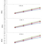Figure 1: Influence of ethanol on brake thermal efficiency at different compression ratios  Click here to view figure

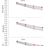Figure 2: Influence of ethanol on brake specific fuel consumption at different compression ratios  Click here to view figure

It is analyzed in Figure 3, the variations of NOx emissions with ethanol gasoline blends as a function of load. NOx emission increases with increase in the load and CR for all test fuels. However, for a given compression ratio, NOx emission reduced with increase in ethanol composition with gasoline. Inherently, the higher rate of evaporation of ethanol brings about cooling effect in the combustion chamber resulting in reduced in-cylinder temperature and in turn reduced NOx production¹⁹. At 100% load, NOx emission at CR 6 for E10, E20, E30 and E40 were found to be 512, 540, 491 and 528 ppm respectively. At 100% load, NOx emission at CR 9 for E10, E20, E30 and E40 were found to be 423, 451, 402 and 439 ppm respectively. The adiabatic flame temperature with ethanol increases with increase in CR and hence the increase in NOx emission at a specific CR. It can be analyzed from Figure 4, the variations of HC emission with all test fuels as a function of load, that HC emissions increases with increase in load. At 100% load, HC emission at CR 6 for E10, E20, E30 and E40 were found to be 43.75, 46.75, 41.75 and 49.25 ppm respectively. Whereas, HC emission at CR 9 for E10, E20, E30 and E40 at 100% load were found to be 30, 33, 28 and 35.5 ppm respectively. At higher CRs, as the engine runs at lean fuel air mixture and thus HC emission decreased as compared with low CR. Figure 5 depicts the variations of CO emission for all test fuels at various CRs. It can be seen for Figure 5 that there is marginal increase in CO emission with increase in the ethanol composition to gasoline or a given CR. However, with increase in CR, CO emission has found to be reduced. At 100% load, CO emission at CR 6 for E10, E20, E30 and E40 were found to be 0.201%, 0.203%, 0.199% and 0.202% respectively. Whereas, CO emission at CR 9 for E10, E20, E30 and E40 at 100% load were found to be 0.035%, 0.037%, 0.033% and 0.036% respectively. The lighter fraction of ethanol in comparison to gasoline tends to achieve almost complete conversion of CO into CO₂.

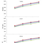Figure 3: Influence of ethanol on NOx emission at different compression ratios Click here to view figure

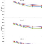Figure 4: Influence of ethanol on HC emission at different compression ratios Click here to view figure

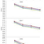Figure 5: Influence of ethanol on CO emission at different compression ratios Click here to view figure

The layout of proposed methodology is presented in Figure 6. ²⁰ The multi – attribute decision making problems in general shall be presented as given in Eq.1.

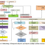Figure 6: Methodology of Integrated subjective and objective multiple attribute decision making  Click here to view figure

A multi attribute decision making method consists of, 1. Alternatives, Ai (for i = 1, 2, … , n), 2. Attributes, Bj (for j = 1, 2, … , m), 3. Weight of each attribute, wj (for j = 1, 2, … , m) and 4. Measures of performance of N number of alternatives w.r.t the attributes, xij (for i = 1, 2,… , n; j = 1, 2, … , m). Generalized structure of MADM²¹ is shown in Table 1.

Table 1: Generalized MADM structure

Alternatives	Attributes
	B1 (w1)	B2 (w2)	B3 (w3)	(-)	(-)	Bm (wm)
A1	X11	X12	X13	–	–	X1m
A2	X21	X22	X23	–	–	X2m
A3	X31	X32	X33	–	–	X3m
–	–	–	–	–	–	–
An	Xn1	Xn2	Xn3	–	–	Xnm

The stepwise procedure of integrated objective and subjective MADM method is presented below

Step 1: Decision table

The attributes of the parameter selection problem are to be chosen in such a way that they satisfy the considered parameter selection problem. These attributes chosen may be either beneficial or non-beneficial and each attribute should be assigned with a qualitative or quantitative value. The attribute with qualitative value should be assigned with a crisp value based on 11 point fuzzy scale²² and the attributes with quantitative values shall be taken directly. In the present study, there are 16 alternatives shown as Trail 1, 2,3, ….. 16. The attributes chosen are 7 which are brake power (BP), brake specific fuel consumption (BSFC), Brake thermal efficiency (BTE), oxides of nitrogen (NOx), hydrocarbon (HC), carbon monoxide (CO), carbon dioxide (CO₂). As the units of attributes are different, normalization of the values of attributes is needed so as to nullify the effect of different units of attributes. The standard normalization procedure was adapted and the normalized values of experimental results are listed as Table 2.

Table 2: Normalized values of experimental results

Trail No.	Normalized values
	BSFC (kg/h kW)	BTE (%)	NOx (ppm)	HC (ppm)	CO (%)	CO2 (%)
1	1.000	0.683	0.636	1.000	1.000	0.522
2	0.984	0.756	0.845	0.864	0.972	0.511
3	0.926	0.881	0.814	0.728	0.931	1.000
4	0.922	0.927	1.000	0.838	0.927	0.500
5	0.603	0.793	0.689	0.792	0.505	0.511
6	0.637	0.744	0.614	0.962	0.560	0.718
7	0.543	1.000	0.848	0.656	0.463	0.500
8	0.565	0.902	0.835	0.809	0.500	0.511
9	0.426	0.881	0.759	0.647	0.220	0.958
10	0.426	0.981	0.898	0.681	0.211	0.451
11	0.465	0.788	0.494	0.860	0.271	0.442
12	0.442	0.850	0.689	0.800	0.239	0.451
13	0.266	0.962	0.801	0.511	0.161	0.442
14	0.290	0.935	0.773	0.579	0.193	0.442
15	0.286	0.895	0.572	0.570	0.188	0.451
16	0.324	0.816	0.477	0.817	0.243	0.442

Step 2: Weight of attributes

Attribute’s weights shall be either the values assigned by the decision maker or results obtained from experiments or assigned based on objective and subjective weights calculated from experimental results. In the present study, objective, subjective and combination of both are considered.

Step 2.1: Objective weights 

Statistical variance is used to determine objective weights as given in Eq. 2.

Where

is taken as normalized value of,

is statistical variance for j^th attribute,

is taken as mean of.

Values of statistical variance for 7 attributes are calculated as given below:

=0.280; =0.159; =0.126; =0.559;         =0.184; =0.186; and =0.484.

Objective weight of j^th attribute,  shall be calculated using Eq. 3 as given below,

Objective weight of j^th attribute, shall be calculated using Eq. 3 as given below,

Objective weights of 7 attributes were calculated and presented as,

Step 2.2: Subjective weights

The subjective weights were determined using analytical hierarchy process and are given as,

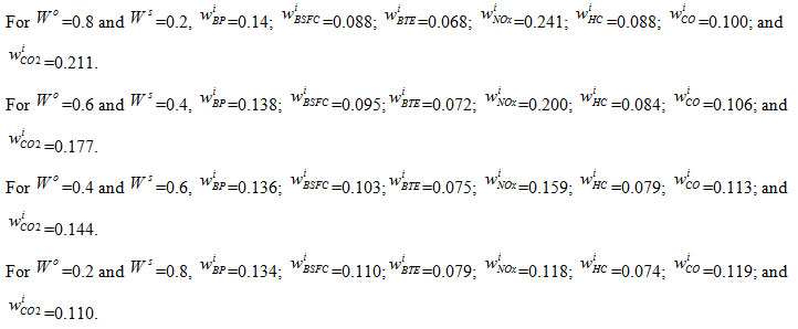
Step 2.3: Integrated weights

Integrated weights, i.e. the combined objective and subjective weights are calculated using Eq. 4.

Where,

is assigned to integrated weight for j^th attribute. Whereas,

and

are denoted as weightings assigned to objective and subjective weights respectively which range between 0 and 1. The integrated weights for attributes such as BP, BSFC, BTE, NO_x, HC, CO and CO₂ calculated in the present study are as follows:

Step 3: Preference index

Given the weights of attributes, the preference index (P) for each alternative considering objective weight alone is calculated using Eq. (5),

Similarly, considering subjective weights alone P is calculated using Eq. (6),

And considering integrated weights, P is calculated using Eq. (7),

Where,

for beneficial attributes,

for non-beneficial attributes,

represent normalized values for beneficial and

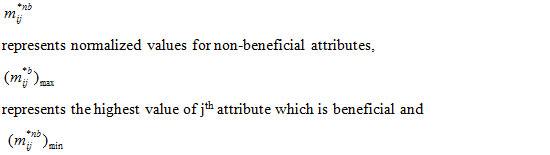
represents the least value of j^th attribute which is non-beneficial. In this study BP, BSFC, BTE are considered as beneficial and NO_x, HC, CO and CO₂ are considered as non-beneficial.

The preference index values for all alternatives are calculated. The preference index for Trail 1 considering objective, subjective and integrated weights are given below as an example:

For objective weight

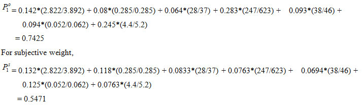
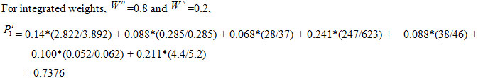
Similarly the preference index for all alternatives considering objective, subjective and integrated weights is calculated.

Step 4: Final selection

The values of preference index calculated for all alternatives are sort and arranged in descending order. Of which, the alternative having highest value of preference index is the best choice from among the considered decision making problem. Practical considerations and constraints may also be taken into account while taking decision. However, compromise can be made towards the alternative with highest preference index. The values of preference index of all alternatives considering objective, subjective and integrated weights are listed in Table 3. It is seen from Table 3 that the preference index for trail 3 is highest by considering objective, subjective and integrated weights. Thus the combination of compression ratio 6, fuel E30 at a load of 75% is found to the best choice from among other trails.

Table 3: Preference index for all trails

Preference Index
Trail No.	Objective weights ()	Rank	Trail No.	Subjective weights()	Rank	Integrated weights
						Trail No.	=0.8 and =0.2	Rank	Trail No.	=0.6 and =0.4	Rank	Trail No.	=0.4 and =0.6	Rank	Trail No.	=0.2 and =0.8	Rank
1	0.742	3	1	0.568	3	1	0.738	4	1	0.690	4	1	0.644	4	1	0.594	5
2	0.656	9	2	0.547	9	2	0.669	9	2	0.637	10	2	0.608	11	2	0.574	11
3	0.764	1	3	0.571	1	3	0.761	1	3	0.712	1	3	0.666	1	3	0.616	1
4	0.750	2	4	0.571	2	4	0.748	2	4	0.699	2	4	0.652	3	4	0.602	4
5	0.694	6	5	0.553	6	5	0.701	7	5	0.664	7	5	0.629	7	5	0.589	7
6	0.645	10	6	0.542	10	6	0.659	12	6	0.627	12	6	0.598	12	6	0.565	12
7	0.609	14	7	0.534	14	7	0.627	16	7	0.598	16	7	0.572	16	7	0.542	16
8	0.619	13	8	0.536	13	8	0.638	13	8	0.611	13	8	0.587	13	8	0.558	14
9	0.704	5	9	0.554	5	9	0.710	5	9	0.670	6	9	0.633	6	9	0.591	6
10	0.674	8	10	0.552	8	10	0.689	8	10	0.651	8	10	0.615	8	10	0.574	10
11	0.634	12	11	0.537	12	11	0.662	11	11	0.636	11	11	0.612	10	11	0.583	8
12	0.638	11	12	0.541	11	12	0.667	10	12	0.638	9	12	0.612	9	12	0.581	9
13	0.726	4	13	0.558	4	13	0.739	3	13	0.697	3	13	0.657	2	13	0.612	2
14	0.685	7	14	0.552	7	14	0.706	6	14	0.672	5	14	0.641	5	14	0.605	3
15	0.592	16	15	0.514	16	15	0.628	15	15	0.605	14	15	0.586	14	15	0.562	13
16	0.596	15	16	0.532	15	16	0.628	14	16	0.605	15	16	0.584	15	16	0.558	15

Comparison of Proposed Method With Graph Theory Matrix Approach

GTMA is a steady and logical approach¹⁵. It has some appealing properties like “ability to model criteria interactions”, “ability to generate progressive models” to show and handle complex issues including attributes with multiple criteria. Results obtained from the proposed integrated objective subjective and integrated approach are compared with GTMA and are listed in Table 4.

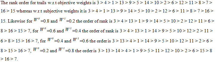
It is seen from Table 4 that parameter index is highest for trail number 3 which is same as that of the proposed method. The order of rank for all trails w.r.t GTMA is 3 > 13 > 12 > 4 > 1 > 6 > 5 > 11 > 14 > 10 > 2 > 9 > 15 >

Table 4: Results of GTMA

Trail No.	CR	Blend	Load (%)	Parameter Index	Rank
						1	6	E10	25	5193	5
2	6	E20	50	3624	11
3	6	E30	75	6998	1
4	6	E40	100	5361	4
5	7	E10	50	4457	7
6	7	E20	25	4681	6
7	7	E30	100	2683	16
8	7	E40	75	3271	14
9	8	E10	75	3349	12
10	8	E20	100	3641	10
11	8	E30	25	3704	8
12	8	E40	50	5741	3
13	9	E10	100	6228	2
14	9	E20	75	3652	9
15	9	E30	50	3349	13
16	9	E40	25	3132	15

8 > 16 > 7. The results of GTMA show that the parameter index for trail number 3 has highest which implies that it is the best choice from among various trails. Thus the proposed mathematical approach is validated. The Spearmann’s rank correlation coefficient has been determined for the proposed method and GTMA. It was found that the Spearman’s coefficient for the proposed method considering objective weights is 0.7291, whereas considering subjective weights it is 1.0000 and considering integrated weights it is 0.9764 for

Conclusion

The experimental investigation on analyzing the influence of ethanol addition to gasoline on performance and emission characteristics of spark ignition engine and a mathematical approach for selection of optimal combination of operating parameters using integrated objective and subjective multi attribute decision making method deduces the following conclusions:

Ethanol gasoline blends make a compatible fuel to spark ignition engine. With increase in compression ratio and increase in composition of ethanol with gasoline, BSFC was found to be increasing. Likewise, BTE increases with increase in ethanol blend and compression ratio.

NOx emission reduced with increase in ethanol composition with gasoline. HC emission reduced with increase in compression ratio. Whereas, CO emission decreased with increase in compression ratio.

The proposed mathematical approach is simple and easy in computation. Nevertheless, it can be adapted to any decision making scenario.

The proposed method can handle any number of alternatives either subjective or objective or both subjective and objective unlike GTMA, which becomes complicated if the number of attributes is more than 20.

The concept of statistical variance infers invaluable information as the variance considers all data points to determine the distribution.

Correlation of ranks for the proposed method and GTMA proves global relevance for solving various complex parameter selection scenarios.

Uniqueness of the proposed method is that, it offers a general system pertinent to different parameter selection scenarios in engineering science and technology.

Acknowledgments

The authors would like to thank Ms. TEENUJA BRIDJESH, for having given the necessary facilities to publish the findings of this research in the form of technical paper. The author also express gratitude to his superiors, peers and colleagues who were instrumental in providing their rich experience, suggestions and guidance which resulted in shaping the technical paper to the current form.

Conflicts of Interest

The authors declare that they have no any conflicts of interest.

References

1. Kasmaei, A. S.; Rofouei, M. K.; Olya, M. E.; Ziaulla. M. Orient J Chem. 2019, 35, 966-972. http://dx.doi.org/10.13005/ojc/350307 Tuner. M. SAE Technical Paper. 2016, 2016-01-0882. https://doi.org/10.4271/2016-01-0882.
2. Chongming, W.; Soheil, Z. R.; Liming, X.; Hongming, Xu. Appl Energy. 2017, 191, 603–619. http://dx.doi.org/10.1016/j.apenergy.2017.01.081
3. Gravalos, I.; Moshou, D.; Gialamas, T.; Xyradakis, P. Renew Energy, 2013, 50, 27-32. doi: 10.1016/j.renene.2012.06.033
4. Kar, K.; Cheng, W.; Ishii, K. SAE Paper No. 2009, 2009-01-1907. https://doi.org/10.4271/2009-01-1907
5. Cooney, C. P.; Worm, J. J.; Naber, J.D. Energy Fuels. 2009, 23, 2319-2324. https://doi.org/10.1021/ef800899r
6. Kim, N.; Cho, S. Automot. Eng. 2014, 158, 725–732. doi:10.4271/2014-01-1208.
7. Nakata, K.; Utsumi, S.; Ota, A.; Kawatake, K. SAE Technical Paper. 2006, 2006-01-3380. https://doi.org/10.4271/2006-01-3380.
8. Szybist, J.; Foster, M.; Moore, W.; Confer. K. SAE Technical Paper. 2010, 2010-01-0619. https://doi.org/10.4271/2010-01-0619.
9. Sari, R.; Golke, D.; Enzweiler, H.; Santos, K. SAE Technical Paper. 2017, 2017-36-0208. https://doi.org/10.4271/2017-36-0208.
10. Milap, G. N.; Amish, P. V. Renewable Energy. 2019, 138, 18-28. https://doi.org/10.1016/j.renene.2019.01.054
11. Dhingra, S.; Bhushan, G.; Dubey, K. K. Mech. Eng. 2014, 9, 81-94. https://doi.org/10.1007/s11465-014-0287-9
12. Pandey, V.; Nikolaidis, E.; Mourelatos, Z. SAE Int. J.Mater. Manuf. 2011, 4, 1155-1168. doi:10.4271/2011-01-1080.
13. N. K.; Pappula. B. SAE Technical Paper. 2019, 2019-01-0025. doi:10.4271/2019-01-0025.
14. Geetha, N. K.; Sekar, P. Sci. Technol. 2018, 21, 7–16. https://doi.org/10.1016/j.jestch.2017.12.011
15. Mustafa, K. B.; Cenk, S. Energy. 2014, 71, 194-201. http://dx.doi.org/10.1016/j.energy.2014.04.074
16. Sari, R. L.; Golke, D.; Enzweiler, H. J.; Salau, N.P.G.; Pereira, F.M.; Martins, M.E.S. Therm. Eng. 2018, 138, 523-533. https://doi.org/10.1016/j.applthermaleng.2018.04.078
17. Boretti, A. SAE Technical Paper, 2010, 2010-01-1453. https://doi.org/10.4271/2010-01-1453
18. Ilves, R.; Kuut, A.; Kikas, T.; Olt, J. Agronomy Research. 2014, 12, 341-350.
19. Thangavelu, S.K.; Ahmed, A.S.; Ani, F.N. Renewable Sustainable Energy Rev. 2016, 56, 820-835. DOI:10.1016/j.rser.2015.11.089
20. Rao, R. V.; Patel, B. K. Materials and Design. 2010, 31, 4738–4747. doi:10.1016/j.matdes.2010.05.014
21. Bridjesh, P.; Periyasamy, P.; Purushothaman, K.; Geetha, N. K. SAE Technical Papers. 2018, 2018-28-0018. doi:10.4271/2018-28-0018
22. Baykasoglu, A. Artif Intell Rev. 2014, 42, 573-605. doi: 10.1007/s10462-012-9354-y

---

This work is licensed under a Creative Commons Attribution 4.0 International License.