Groundwater Quality of Coastal Aquifer Evaluation Using Spatial Analysis Approach

Introduction

Assessment of groundwater quality of a region is essential to plan for proper groundwater utilization and development (Singh et al., 2009). Day by day increasing groundwater demand for domestic uses industrialisation and agricultural production require continuous monitoring of groundwater quality (Rawat et al., 2017a, Rawat et al., 2018a, b). The declination of groundwater quality affects its usage for domestic, industry and agricultural activities (Amin et al., 2013; Bharose et al., 2013; Choudhary et al., 2013; Gupta et al., 2014; Jacintha et al., 2016; Nemcˇic´-Jurec et al., 2017). After the detection of contamination factors, it is often difficult to carry out a proper planning to overcome the poor groundwater quality. Hence, it is essential that the regular monitoring of groundwater quality to proper utilization of groundwater resources. Techniques namely multivariate statistical analysis, remote sensing and Geographic Information System (GIS) are evolving to evaluating and possibility of exploring of groundwater contamination sources (Kumar et al., 2015; Rawat et al., 2017a, Rawat et al., 2018a; Rawat et al., 2018b; Rawat et al., 2017b; Rawat et al., 2018c; Rawat et al., 2018d). GIS is one of them a powerful tool for finding solutions for groundwater resource management problems such as evaluation of groundwater quality with respect to the number of features of the study area such as geology, land use (Anbazhagan and Nair, 2004; Babiker et al., 2007; Vijith and Satheesh 2007; Voudouris, et al., 2010; Ketata, et al., 2011 Srinivasamoorthy et al., 2011; Sharma et al., 2018; Thakur et al., 2016), identifying groundwater potential zones (Rai et al., 2005; Rao, 2006; Chenini et al., 2010; Preeja et al., 2011), etc. GIS is a dynamic and strong tool (Rawat et al., 2012; Rawat et al., 2013; Rawat et al, 2018a, b) for GWQ mapping and important for monitoring environmental changes (Engay 2015; Guzman et al., 2010). Water Quality Indices (WQIs) are commonly used tool in assessment of groundwater quality; it summarizes a number of groundwater quality elements into an important single numerical values (Stambuk-Giljanovik, 2003; Singh, & Gautam, 2016; Singh et al., 2017a, b). It is very simple for decision makers to know about groundwater quality using WQI (Jacintha et al. 2016). The present study was carried out in a part of coastal aquifer of Thiruvallur district, Tamil Nadu, India, region where. This region is characterized by concentration of groundwater by sea water mixing process (Balasubramanian et al. 1985; Gnanasundar and Elango, 1999). To manage groundwater resources sustainably, it is important to analyzed all GWQ parameters together for an integrated approach is very useful for evaluating and solving the problem. With this target, the present study aims to fill the gap in previous studies of the area and to assess the groundwater quality based on eight parameters ((Hydrogen–ion activity (pH), Alkalinity, Hardness, Fluoride, Iron, Ammonia, total Nitrate (NO₂+NO₃), and Residual Chloride in a part of Chennai Metropolitan area, TamilNadu (India).

Study Area

The Chennai Metropolitan area extends over 1189 km² and the city area is 426 km². The study area is extending over an area of 87.25 km² (Fig. 1) with the perimeter of 57.35 km. The study area is bounded by the Koovam river in North, Adyar river in South, Bay of Bengal Coast in East and the city boundary in West.The study area is located between North Latitude13°4’55.98″ and 13° 0’7.50″ and between East Longitude 80°17’22.37″ and 80° 8’42.20″ with the elevation varying between 5m above mean sea level near the coast to about 15m in the western boundary (Fig. 1). It forms part of the Survey of India (SOI) Topographic sheet 66 C/1 and 66 C/4. As the area fall in-between two streams i.e., Adyar and Koovam. Both these streams have deposited substantial amount of alluvium–mixture of sand sit and claythat forms an important aquifer in the Chennai city.

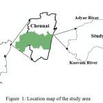Figure 1: Location map of the study area. Click here to View figure

 

Geologically, the alluvial deposits rest on hard rock on the eastern and southern parts. The hard rock is mainly charnockites of Archaean age. In the northern and western part, the alluvium rests over tertiary and gondwana group of rocks. The average thickness of alluvium varies from 10m along the southern boundary to a maximum of 30 m in the central and eastern part of the study area.

Shallow open dug wells of depth varying from 8 m to 10 m and borewells in the depth range of 30 m to 75 m are the common groundwater extraction structures in the area (Saravanan et al., 2018). The Total Dissolved Solids of the open-well water varies between 500 to 1500 mg/l and that of the borewells vary from 1000 to 2000 mg/l.

Climate and Rainfall

The Metropolitan area enjoys a tropical climate. The period from April to June is generally hot and from December to February is pleasant. The mean annual temperature is 24.3 (min) to 32.9°C (max). The extreme temperatures recorded are 13.9and 45°C. The humidity is generally high and the percentage of humidity ranges between 58 and 84. Chennai receives the major part of the rainfall during the north-east monsoon period in the months of October, November and December. The south-west monsoon rainfall between June and September is generally erratic and the summer rains are negligible (Saravanan et al., 2018). The normal annual rainfall recorded in the Meenambakkam Observatory is 1323.7 mm and in the Nungambakkam Observatory is 1285.6mm. Around 60% of the annual rainfall is contributed from northeast monsoon, 30 % from southwest monsoon and the balance of around 10% is contributed from winter and summer rainfall.

Materials and Methods

Survey of topographic map (scale 1:50,000) was used forpreparation of the base map. Groundwater samples were collected from dug bore and bore wells in the study area in October 2015. The water quality parameters were analyzed using the test kit obtained from Tamil Nadu Water Supply and Drainage Board. The parameters analyzed include, pH, Alkalinity, Hardness, Fluoride, Iron, ammonia, total Nitrate (NO₂+NO₃), and Residual Chloride Further, suitability of water for drinking purposes has been checked. In additional water levels data were also observe during February (pre-monsoon) and August 2015 (post- monsoon).

Inverse Distance Weighting (IDW)

In interpolation with IDW, a weight is attributed to the point to be measured. The amount of this weight is dependent on the distance of the point to another unknown point. These weights are controlled on the bases of power of ten. With an increase of power of ten, the effect of the points that are farther diminishes. Lesser power distributes the weights more uniformly between neighbouring points. In this method the distance between the points count, so the points of equal distance have equal weights (Burrough and McDonnell, 1998). The weight factor is calculated with the use of the following formula eqn. (1):

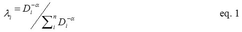
λ_i, weight of point; D_i, a distance between point i and the unknown points; α, the power ten of weight.

The advantage of IDW is that it is intuitive and efficient. This interpolation works best with evenly distributed points. Similar to the SPLINE functions, IDW is sensitive to outliers. Furthermore, unevenly distributed data clusters result in introduced errors.

Determination of WQI

Nemerow’s pollution index (NPI or WQI) is a simplified pollution index introduced by Neme (Mohan et al., 2007) which is also known as Raw’s pollution index. It is given as

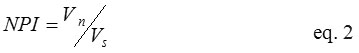
Where, V_n = Actual value or observed concentration of n^th parameter; V_{s =} permissible limit of n^th parameter.

Overlay Analysis

Overlay analysis using in GIS platform for proposing groundwater quality map depending on a number of thematic layers on the special information of study area. In overlay analysis at pixel level each individual pixel of each layers/raster (X_n) is multiplied by a weight (W_n, from eqn. 1 and 2) to assign new value to each and finally add each layer for the final index value for each pixel of every location on the map; this can be interpreted by eqn. (4) (Eastman, 2001).

NPI or WQI=∑ NPI_n                                      eq.3

where, WQI index for each pixel in the n^th parameter’s map

The total NPI score of each pixel of the final integrated layer (after overlay analysis) were derived from the following eq. (5):

NPI or WQI=NPI_pH+NPI_Alkalinity+NPI_TH+ NPI_Cl+ NPI_F+NPI_Fe+NPI_NH4+NPI_NO3                       eq.4

where, the subscript letter represents a parameter, W represents the weight of correspondent subscript parameter. X is thematic layers of a correspondent subscript parameter.

Thus, the groundwater quality index (WQI), which is dimensionless quantity that helps in indexing the probable groundwater quality zones in the area, was estimated using eq. (4) for each pixel in the final integration layer of WQI and was categorized into different classes into different WQI zones within study area.

Results and Discussion

The observation wells are shallow openwells varying depth from 6 m to 10 m below ground level mapping mainly from the alluvial formation which forms the major aquifer in the area. In all 96, wells have been located in the study area. About 17 (17.7%) wells fall just outside the boundary of the study area; this was due to the fact that the same aquifer extends in these areas and to assess the variation just outside the boundary also. All the wells have been geo-coded and a base map has been prepared. The water samples were collected during February 2015–representing post monsoon and in and August 2015 during monsoon. 2014 was a normal rainfall year with about 1294 mm which should get reflected in the February data. The August 2015 data should reflect the quality during the south east monsoon (July to September). The rainfall received upto August 2015 is about 350 mm.  In fact in 2015, the rainfall was above normal during which the city got flooded due to heavy deluge and the month of November, receiving about 1013 mm in that month itself.

During Feb 2015, the pH values in the wells were observed to vary from 6.5 to 8. In 91 (94.8%) wells, the pH is between 6 and 8.5 (Table 1). The Acceptable and Permissible limit as per WHO-2006. Drinking water quality standards, it should be between 7 and 8.5 (Table 1). In the study area, the values fall within the limits (Fig. 2a). During Aug-2015, the pH value in the wells was observed to vary from 6.5 to 8. In 2 wells it is 6.5, and in the rest of the wells it ranges from 7–8 and is within the standards.

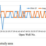Figure 2a: pH concentration over study area. Click here to View figure

 

The alkalinity of the water seems to vary from 200–500 mg/l. The acceptable limit (as WHO-2006) for alkalinity is 200 mg/l (Table 1) while the permissible limit is 600 mg/l. hence in this case, though the water samples are above the acceptable limit, it found to be within the permissible limit (Fig. 2b). While water samples during Aug 2018 seems to vary from 100–600mg/l. In 17 (17.7%) wells it is within (200 mg/l) acceptable limit and remaining are in the rest it is within the permissible limit (Fig. 2b).

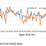Figure 2b: Alkalinity concentration over study area. Click here to View figure

 

The hardness of the water samples from open wells seems to vary from 150–560mg/l. The acceptable limit for hardness is 200 mg/l (Table 1) and the permissible limit is 600 mg/l. Based on this parameter, about 13 (13.54%) wells are within the acceptable limit (as WHO-2006) while the remaining are within the permissible limit (Fig. 2c). And during monsoon hardness of the sample seems to vary from 110–640mg/l (Fig. 2c). The higher values above the permissible limit are observed in 3 (3.13%) locations in areas such as MMDA Colony, Manapakkam and Mugalivakkam where in the alluvium overlie the Gondwanas.

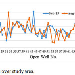Figure 2c: Hardness concentration over study area. Click here to View figure

 

The Chloride of the water seems to vary from 20–400mg/l. The acceptable limit is 250 mg/l (Table 1) and the permissible limit is 1000 mg/l. The basis of chloride factor, about 76 (79.17%) wells is within the acceptable limit (Fig. 2d). The chloride of the collocated water samples vary from 90–800mg/l (during 2015 monsoon period) with about 50 (52.08%) wells are within the acceptable limit. The higher value of 800mg/l was noticed in Theosophical society located to the south of Adyar river during monsoon (Fig. 2d).

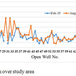Figure 2d: Chloride concentration over study area. Click here to View figure

 

Fluoride concentration in the study area varies from nil (≈0) to 2 mg/l. It was nil in 25 (26.04%) samples while less than/equal to 1 in 85 (88.54%) wells. In just one sample it is measured as 2 mg/l in observation open well no. 2 in Muggappair West falling outside the study area. The acceptable limit is 1.5 (Table 1). The basis of WHO-2006 limit almost 90 % of the wells are within permissible limit while remaining 10 % is within the acceptable limit during pre-monsoon (Fig. 2e), while Fluoride during monsoon varies from 0–2mg/l. Fluoride reported nil in 16.67% samples, and less than or equal to 1 in 41.67% water samples. In just two samples it is measured as 2 mg/l observed at Anna Nagar and in South Boag Road, T. Nagar.

Table 1: Descriptive statistics of hydro-chemical data of groundwater samples from open wells at study area during (a) Feb-2015, pre-monsoon and (b) Agu-2015, post monsoon.

a
		pH	Alkalinity	Hardness	Chloride	Fluoride	Iron	Ammonia	NO2+NO3
ST		8.5	200	200	250	1.5	0.3	0.5	45
Min		6	200	150	20	0.00001*	0.00001*	0.00001*	0.00001*
Max		8	500	560	400	2	15	5	46
Ran		2	300	410	380	1.99	14.99	5	46
S		686.5	30340	27670	18280	50.4	55	44.8	1815.1
Me		7.2	319.4	291.3	192.4	0.5	0.6	0.5	18.9
Med		7	310	290	190	0.5	0.3	0	15
Mo		7	310	310	170	0.5	0.00001*	0.00001*	15
SD		0.3	63.9	73.2	72.7	0.5	1.9	0.9	11.7
Vari		0.1	4078.0	5358.0	5287.0	0.2	3.7	0.8	137.9
IQR		0.5	100.0	95.0	100.0	0.5	0.3	0.0	13.1
SoS		8.6	383400	503600	496900	20.6	354.8	77.2	13100.
MAD		0.2	52.4	56.2	57.0	0.3	0.7	0.6	9.1
RMS		7.2	325.6	300.2	205.6	0.7	2.0	1.0	22.2
SEM		0.0	6.6	7.5	7.5	0.0	0.2	0.1	1.2
Sk		0.1	0.2	0.4	0.4	0.9	5.8	2.5	0.5
K		4.7	2.6	3.8	3.2	3.4	39.2	10.0	3.1
CoV		0.0	0.2	0.3	0.4	0.9	3.4	1.9	0.6
RS (%)		4.2	20	25.1	37.8	88.78	337.3	193.1	62.1
b
Min	6.5		100	110	90	0.00001*	0.00001*	0.00001*	15
Max	8		600	640	800	2	1.5	3	45.2
Ran	1.5		500	530	710	2	1.4999	3	30.2
S	698		29900	30790	26120	91.5	22.1	23.5	2268.8
Me	7.3		311.5	320.7	272.1	1.0	0.2	0.2	23.63
Med	7.5		310	310	245	1	0.00001*	0.00001*	20.2
Mo	7.5		360	310, 300	180	1.5	0.00001*	0.00001*	20.2
SD	0.3		101.5	113.4	132.7	0.6	0.4	0.5	7.7
Vari	0.1		10300.0	12870.0	17620.0	0.3	0.2	0.3	58.8
IQR	0.5		150.0	130.0	140.0	1.0	0.0	0.0	0.2
SoS	7.5		978200	1222000	1674000	32.0	18.8	25.5	5584.0
MAD	0.3		82.7	84.8	97.6	0.5	0.4	0.3	5.4
RMS	7.3		327.4	340.0	302.4	1.1	0.5	0.6	24.8
SEM	0.0		10.4	11.6	13.6	0.1	0.0	0.1	0.8
Sk	-0.3		0.2	0.8	1.5	-0.4	1.6	3.9	2.1
K	2.3		2.8	3.7	5.5	1.8	4.2	19.6	5.9
CoV	0.0		0.3	0.4	0.5	0.6	1.9	2.1	0.3
RS (%)	3.85		32.58	35.37	48.78	60.93	193.40	211.70	32.44

 

ST, Slandered Value (as WHO-2006); Min, Minimum; Max, Maximum; Ran, Range; S, Sum; Me, Mean; Mo, Mode; SD, Standard Deviation; Vari, Variance; IQR, Interquartile Range; SoS, Sum of Squares; MAD, Mean Absolute Deviation; RMS, Root Mean Square; SEM, Std Error of Mean ; Sk, Skewness; K, Kurtosis; Cov, Coefficient of Variation; RS, Relative Standard Deviation; “*” is negligible value (≈0). Except pH all parameters concentration or measured unit is mg/l.

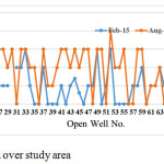Figure 2e: Fluoride concentration over study area. Click here to View figure

 

Iron in the open wells water sample varies from nil (≈0) to 15 mg/l while the acceptable and permissible limit for iron is 0.3 mg/l (Table 1, Fig. 2f). If iron exceeds the 0.3 mg/l, it leads to the yellow colouration of water, increases turbidity, and water could not be used for direct consumption without removal systems. Higher concentration promotes iron bacteria. In the study area, it is nil in 45.8% (44) collected samples, upto 0.3 mg/l in 31.25% (30) samples; higher concentration of 1mg/l and above is observed in 8 open wells that mainly in the western part of the study area like in Koyambedu, Arumbakkam and in Ashok nagar where iron bearing clay lenses are quite common. One sample observed in Theosophical society showed the highest concentration of 15 mg/l. is due to the presence of iron bearing clay and sand in this area. During monsoon iron in the water sample vary from 0–1.5mg/l. It found zero concentration in 76.04% (73) samples. Andrang of 0.3–1.0 mg/l in 17 (17.7%) samples ramming 4.17% (4) water samples come under 1.5 mg/l limit during 2015 monsoon period. In comparison of pre-monsoon (Feb-2015),iron concentration reduced with falling water table in the study area during monsoon (Agu-2015).

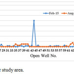Figure 2f: Iron concentration over study area. Click here to View figure

 

Ammonia in the open wells water sample follows range of 0–5 mg/l (Fig. 2g). The acceptable and permissible limit of Ammonia is 0.5 mg/las WHO-2006 (Table 1), and the presence of ammonia beyond of the limits is an indication of faecal contamination of the water. In the study area, it was nil in 59.38% (=57) samples and 9.38% (=9) samples come in 0.3 mg/l. While a higher concentration of > 0.5mg/l of Ammonia was observed in 30.21% (=29) samples (Fig. 2g) during pre-monsoon. But during monsoon higher concentration (> 0.5 mg/l) of Ammonia was reduced and only 4 wells found under higher concentration limit (Fig. 2g). From fig. 2g, it is clear 55.21% (53) water sample follow concentration range of 0–3mg/l.

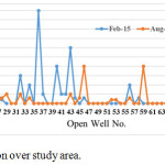Figure 2g: NO2+NO3 concentration over study area. Click here to View figure

 

Total Nitrate in the water sample from open wells of study area come under range of 0–45mg/laccording to fig.2h during pre-monsoon. The permissible limit of this factor is 45 mg/l (WHO-2006). Presence of Nitrate above the limit is an indication of pollution of the water. In the study area, three categories of concentration were found for total nitrate, namely 0 (9.38% sample), < 10 (15.63% sample), and 45 mg/l (remaining samples).

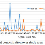Figure 2h: Total Nitrate (NO3+NO2) concentration over study area. Click here to View figure

 

In order to the analysis of the groundwater quality variation with respect to water level, the water levels observed during February and August 2015 is presented in Fig 3. Interestingly, the water level in August 2015 (average at 5.66 m below ground level (bgl)), i.e., during South West monsoon, is almost 1.5m below the levels as compared to Feb 2015 (average at 4.07 mbgl). To correlate the quality data, the samples were analyzed during August 2015. The groundwater level and groundwater quality analysis reveal that category of 5.1–10.0 (good) is increasing in comparison of Feb 2015 while range of 10.1–15.0 (moderate), 15.1–20.0 (poor), and 20.0 < (unsuitable for drinking use), vanished in Aug- 2015 (Fig.4a). Fig. 4b revealed rainfall effect over groundwater quality of the study area during pre- monsoon and monsoon period of 2015. According to Fig. 4b, due to rainfall 9(or 9 % of total open wells) open wells of excellent category converted into good because of adding of some contention from soil leaching process. During monsoon, 15 (or 15.63 %) open wells were more from pre-monsoon 2015 in a good category of water, while 2.1 % more from pre-monsoon open wells come under permissible limit during monsoon may be due to some geo-chemistry process.

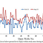Figure 3: Water level (in m below ground level (bgl)) within study area during study period. Click here to View figure

 

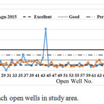Figure 4a: NPI/WQI values for each open wells in study area. Click here to View figure

 

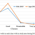Figure 4b: Number of open wells in each class with in study area during 2015. Click here to View figure

 

On the basis of statistics analysis, almost 33 and 24 percent of total open wells water samples are having rank 1 (excellence) during pre-monsoon (Feb-2015) and monsoon (Agu-2015) respectively while percentage of the total number open well under second class (or good class) are increased (which is 68.8 percent) during the monsoon period. These statistics show study area has ideally come under rank 2 or class of good. Thus, the groundwater quality of this study area is fit or can use without treatment for domestic purposes. Overall, 4% of the open wells water is affected and majority of contamination by sea and river water mixing process within the study area because from three side study area surround by sea and polluted monsoon river. The groundwater quality of a region depends on severalcauses including land use, slope, geology topography, etc. In this research, groundwater quality of water fordrinking purposes was assessed based on the water quality parameters. In order to understand whether there is anyinfluence of land use, slope, geology topography, etc of the region, a comparison study was performed among these parameters and groundwater quality map. It is generally assumed that, land use, ground slope, geology topography controls the groundwater recharges processes which will influence the groundwater quality. Such evidences however was not found in this site (may be due to one year data for analysis).

Integrated Groundwater Quality Mapping

Figure 4c and 4d show the final drinking water quality maps that were produced by integrating eight thematic layers. pH, Alkalinity, Hardness, Fluoride, Iron, ammonia, Nitrite+Nitrate (total), and Residual Chloride. The spatial integration for groundwater quality mapping was carried out using overlay analysis. It can be seen in the final drinking groundwater quality map based on Raw’s pollution index (Mohan, et al., 2007) and WHO (2006) permissible limits for parameters. The groundwater quality mapping of this area was achieved by assigning weightage to eight parameters (as mentioned by eq. 2). Table 3, a rank/class 1, of <5 (light Grace colour patches) reveals that groundwater is excellent for domestic use where as a rank/class2, of 5.1–10.0(Yellow colour patches) represent good than class 3^th indicates (10.1–15.0) moderated/permissible (Green colour patches)in use, while fourth (15.1–20.0, Blue colour patches) and fifth (20.1 <, Red colour patches) class represent to poor and unsuitable for drinking, respectively.

Table 2: Classification of water quality on the basis of WQI/NPI.

WQI	Class/Rank
< 5.0	Excellent
5.1-10.0	Good
10.1-15.0	Poor
15.1-20.0	Very poor
20.1 <	Unsuitable for drinking

 

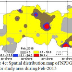Figure 4c: Spatial distribution map of NPI/GWQ map for study area during Feb-2015. Click here to View figure

 

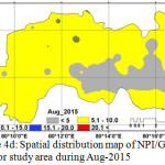Figure 4d: Spatial distribution map of NPI/GWQ map for study area during Aug-2015. Click here to View figure

 

Conclusion

After the overlay analysis of eight groundwater parameters for potable and non-potable zones in the study area, the final groundwater quality maps were derived. As can be seen from the map some regions have groundwater that is required proper treatment before using. The statistical and spatial variability analysis of groundwater (from open wells) quality in the study area has revealed that most of the sampling locations are matches with the permissible limit of drinking water quality as prescribed by the WHO-2006. These maps provide public, local administrator and the government to be aware of crisis of poor water quality. Present status of groundwater of study area requires regular monitoring. Further, groundwater quality declines and strategies for improving the same in future are required. Our recommendations for the region are as (i) proper disposal/recycling of domestic sewage will help in minimizing groundwater pollution by sewage, (ii) development of n number of rainwater harvesting-recharging structures and (iii) regular monitoring of groundwater table level along with groundwater quality of study will minimize the chances of further decline.

Acknowledgement

The authors wish to acknowledge Dr. A.K. Mishra, Principal Scientist, Water technology Center, IARI New Delhi, and Mr. K. Santhanam, Ex. Deputy Director, PWD – Groundwater, Chennai for the support rendered for the successful completion of the work.

References

1. Amin, A.; Fazal, S.; Mujtaba, A.; Singh, S.K.; Effects of land transformation on water quality of Dal lake, Srinagar, India. J Indian Soc Remote Sens. 2014, 42:119–128.
   CrossRef
2. Anbazhagan, S.; Nair, A.M.; Geographic Information System and Groundwater Quality Mapping in Panvel Basin, Maharashtra, India. Environ. Geol. 2004, 45, 753–761.
   CrossRef
3. APHA (1996) Standard methods for examination of water and waste water, 19th edn. Washington DC
4. Babiker, I.S.; Mohamed, M.A.A.; Hiyama, T.; Assessing Groundwater Quality Using GIS. Water Resour. Manage. 2007, 21, 699–715.
   CrossRef
5. Balasubramanian, A., Sharma, K.K.; Sastri, J.C.V.; Geoelectrical and hydrogeochemical evaluation of coastal aquifers of Tambraparni basin, Tamil Nadu, Geophys. Res. Bull. 1985, 23(4):203-209.
6. Bharose, R.; Singh, S.K.; Srivastava, P.K.; Heavy metals pollution in soil-water-vegetation continuum irrigated with groundwater and untreated sewage. Bull Environ Sci Res. 2013, 2:1–8.
7. Burrough, P.A.; McDonnell, R.A.; Creating continuous surfaces from point data. In: Burrough PA, Goodchild MF, McDonnell RA, Switzer P, Worboys M (Eds.). Principles of Geographic Information Systems. 1989, Oxford University Press, Oxford, UK.
8. Chenini, I.; Mammou, A.B.; May, M.E.; Groundwater Recharge Zone Mapping Using GIS-based Multi-criteria Analysis: A Case Study in Central Tunisia (Maknassy Basin). Water Resour. Manage. 2010, 24, 921–939.
   CrossRef
9. Chaudhary, M.P., Uddin, S.; Singh, S.K.; Singh, P.; Statistical analysis for presence of chloride in water at different locations of upper lake in Madhaya Pradesh state of India. Int J Math Arch. 2013, 4:35–37.
10. Engay, K. G., Land Cover Change in the Silang-Santa Rosa River Subwatershed , Laguna, Philippines. Journal of Environmental Science and Management 2015, 18 (6): 34–46.
11. Gnanasundar and Elango, Groundwater quality assessment of a coastal Aquifer using geoelectrical techniques, Journal of Environmental Hydrology, 1999, 7(2),1-8.
12. Guzman, J.B.; Eduardo, P.P.; Antonio, J.A.; A Geographic Information Systems-Based Decision Support System for Solid Waste Recovery and Utilization in Tuguegarao City, Cagayan, Philippines. Journal of Environmental Science and Management, 2010, 13 (6): 52–66.
13. Gupta, L.N; Avtar, R.; Kumar, P.; Gupta, G.S.; Verma, R.L.; Sahu, N.; Sil, S.; Jayaraman, A.; Roychowdhury, K.; Mutisya, E.; Singh, S.K.; A multivariate approach for water quality assessment of river Mandakini in Chitrakoot, India. J Water Resour Hydraul Eng. 2014, 3:22–29.
14. Herman and Bower.; Groundwater Quality, Groundwater  Hydrology, Mc.Graw­Hill Kogakusha Ltd., Tokyo, 1978, pp. 339­375.
15. Jacintha, T.G.A.; Rawat, K.S.; Mishra, A.; Singh, S.K.; Hydrogeochemical characterization of groundwater of peninsular Indian region using multivariate statistical techniques. Appl Water Sci. 2016, 7(6):3001–3013. doi/10.1007/s13201-016-0400-9
16. Ketata, M.; Gueddari, M.; Bouhlila, R. Use of Geographical Information System and Water Quality Index to Assess Groundwater Quality in El Khairat deep aquifer (Enfidha, Central East Tunisia). Arabian J. Geosci. 2011. DOI: 10.1007/s12517-011-0292-9.
    CrossRef
17. Kumar, R.P.; Ranjan, R.K.; Ramanathan, A.L.; Singh, S.K.; Srivastava, P.K.; Geochemical modeling to evaluate the mangrove forest water. Arab J Geosci. 2015, 8:4687–4702.
    CrossRef
18. Nemcˇic´-Jurec, J.; Singh, S.K.; Jazbec, A.; Gautam, S.K.; Kovac, I.; Hydrochemical investigations of groundwater quality for drinking and irrigational purposes: two case studies of Koprivnica-Krizˇevci County (Croatia) and district Allahabad (India). Sustain. Water Resour. Manag. 2017; https://doi.org/10.1007/s40899-017-0200-x
19. Preeja, K.R.; Joseph, S.; Thomas, J.; Vijith, H.; Identification of Groundwater Potential Zones of a Tropical River Basin (Kerala, India) Using Remote Sensing and GIS Techniques. J. Indian Soc. 2011, 39(1): 83-94.
    CrossRef
20. Rai, B.; Tiwari, A.; Dubey, V.S.; Identification of Groundwater Prospective Zones by Using Remote Sensing and Geoelectrical Methods in Jharia and Raniganj Coalfields, Dhanbad District, Jharkhand state. J. Earth Syst. Sci. 2005, 114 (5), 515–522.
    CrossRef
21. Rao, N.S. Groundwater Potential Index in a Crystalline Terrain Using Remote Sensing Data. Environ. Geol. 2006, 50, 1067–1076.
    CrossRef
22. Rawat, K.S.; Mishra. A.K.; Sehgal, V.K.; Tripathi, V.K.; Spatial Variability of Ground Water Quality in Mathura District (Uttar Pradesh, India) with Geostatistical Method. International Journal of Remote sensing Application, International, 2012, 2(1), 1-9.
23. Rawat, K.S.; Mishra, A.K.; Sehgal, V.K.; Tripathi, V.K.; Identification of Geospatial Variability of Fluoride contamination in Ground Water of Mathura District, Uttar Pradesh, India. Journal of Applied and Natural Science, 2013, 4(1), 117-122.
    CrossRef
24. Rawat, K.S.; Tripathi, V.K.; Singh, S.K.; Groundwater quality evaluation using numerical indices: a case study (Delhi, India). Sustain. Water Resour. Manag. 2017a, https://doi.org/10.1007/s40899-017-0181-9
25.  Rawat, K.S.; Mishra, A.K.; Singh, S.K.; Mapping of groundwater quality using Normalized Difference Dispersal Index of Dwarka sub-city at Delhi National Capital of India. ISH J Hydraul Eng. 2017b. 5010:1–12.
26. Rawat, K.S.; Jeyakumar, L.; Singh, S.K.; Tripathi, V.K.; Appraisal of groundwater with special reference to nitrate using statistical index approach. Groundwater for Sustainable Development. 2018a, https://doi.org/10.1016/j.gsd.2018.07.006
27. Rawat, K.S.; Jacintha, T.G.A.; Singh, S.K.; Hydro-chemical Survey and Quantifying Spatial Variations in Groundwater Quality in Coastal Region of Chennai, Tamilnadu, India – a case study. Indonesian Journal of Geography.  2018b, 50 (1): 57 – 69. http://dx.doi.org/10.22146/ijg.27443
    CrossRef
28. Rawat, K.S.; Jacintha, T.G.A.; Singh, S.K.; Hydro-chemical Survey and Quantifying Spatial Variations in Groundwater Quality in Coastal Region of Chennai, Tamilnadu, India – a case study. Indonesian Journal of Geography.  2018c 50 (1): 57 – 69. http://dx.doi.org/10.22146/ijg.27443
    CrossRef
29. Rawat, K.S.; Singh, S.K.; Water Quality Indices and GIS-based evaluation of a decadal groundwater quality. Geology, Ecology, and Landscapes. 2018d, 1-12. https://doi.org/10.1080/24749508.2018.1452462
30. Rawat, K.S.; Singh, S.K.; Jacintha, T.G.A.; Nemcˇic´-Jurec, J.; Tripathi, V.K.; Appraisal of long term groundwater quality of peninsular India using water quality index and fractal dimension. J. Earth Syst. Sci. 2018e, https://doi.org/10.1007/s12040-017-0895-y
31. Saravanan, J.; Rawat, K.S.; Singh, S.K.; Study of Sub Surface Hydrogeology of Chennai Metropolitan Area. Curr World Environ, 2018, 13(3). Available from: http://www.cwejournal.org/article/1254/
32. Shanthi, K.; Ramaswamy, K.; Pramalsamy, P.; Hyderobiological study of Signanallur taluk, at Coimbatore, India, Nature Environ. Pollut. Technol., 2002, 1(2): 97-101.
33. Shivakumar R.; Mohanraja R.; Azeez PA. (2000). Physico-chemical analysis of water source of Ooty, South India. Pollut. Res., 19(1): 143-146.
34. Sharma, B.; Kumar, M.; Denis, D.M.; Singh, S.K.; Appraisal of river water quality using open-access earth observation data set: a study of river Ganga at Allahabad (India). Sustainable Water Resources Management. 2018, 1-11. https://doi.org/10.1007/s40899-018-0251-7
35. Singh, S.; Singh, C.; Kumar, K.; Gupta, R.; Mukherjee, S.; Spatial-temporal monitoring of groundwater using multivariate statistical techniques in Bareilly district of Uttar Pradesh, India. J Hydrol Hydromechanics. 2009, 57:45–54.
36. Singh, H.; Pandey, R.; Singh, S.K.; Shukla, D.N.; Assessment of heavy metal contamination in the sediment of the River Ghaghara, a major tributary of the River Ganga in Northern India. Applied Water Science. 2017a, 7(7):4 133-4149
37. Singh, H.; Singh, D.; Singh, S.K.; Shukla, D.N.; Assessment of river water quality and ecological diversity through multivariate statistical techniques, and earth observation dataset of rivers Ghaghara and Gandak, India. Int J River Basin Manag. 2017b, 15(3): 347-360. https://doi.org/10.1080/15715124.2017.1300159
    CrossRef
38. Smith, K.; Environment hazards: Assessing risk and reducing disaster (3 ed., 2001, pp: 324). London: Routlege.
39. Srinivasamoorthy, K.; Vijayaraghavan, K.; Vasanthavigar, M.; Sarma, V.S.; Rajivgandhi, R.; Chidambaram, S.; Anandhan, P.; Manivannan, R. Assessment of Groundwater Vulnerability in Mettur Region, Tamilnadu, India using drastic and GIS Techniques. Arabian J. Geosci. 2011, 4 (7–8), 1215–1228.
    CrossRef
40. Thakur JK, Singh SK, Ekanthalu VS. 2016. Integrating remote sensing, geographic information systems and global positioning system techniques with hydrological modeling. Appl Water Sci. 2017, 7(4): 1–14.
    CrossRef
41. Vijith, H.; Satheesh, R.; Geographical Information System Based Assessment of Spatiotemporal Characteristics of Groundwater Quality of Upland Sub-watersheds of Meenachil River, Parts of Western Ghats, Kottayam District, Kerala, India. Environ. Geol. 2007, 53, 1–9.
    CrossRef
42. Voudouris, K.; Kazakis, N.; Polemio, M.; Kareklas, K.; Assessment of Intrinsic Vulnearabilit Using the DRASTIC Model and GIS in the Kiti aquifer, Cyprus. European Water. 2010, 30, 13–24.

---

This work is licensed under a Creative Commons Attribution 4.0 International License.