Numerical study and simulation of nano-bubble formation with CFD
Hamid Reza Ghorbani1*, Vahid Ghorbani2
1Department of Chemical Engineering, Qaemshahr Branch, Islamic Azad University, Qaemshahr, Iran
2Department of mathematical, Garmsar Branch, Islamic Azad University, garmsar, Iran
DOI : http://dx.doi.org/10.13005/ojc/300350
Article Received on :
Article Accepted on :
Article Published : 26 Aug 2014
In recent years, microbubble and nanobubble technologies have drawn great attention due to their wide applications in many fields of science and technology, such as water treatment, biomedical engineering, and nanomaterials. In this work, we numerically studied nano-bubble formation process by entering air into a submerged orifice in a cylindrical vessel. The simulations were carried out using SOLA-VOF method. In this code, complete form of Navier-stocks equations was predicted two dimensions and using finite difference method. In addition, the effect of air flow rate on the nano-bubble size and its formation time at very low rates was studied.
KEYWORDS:Nano-bubble; Simulation; CFD; Two phases
Download this article as:| Copy the following to cite this article: Ghorbani H. R, Ghorbani V. Numerical study and simulation of nano-bubble formation with CFD. Orient J Chem 2014;30(3). |
| Copy the following to cite this URL: Ghorbani H. R, Ghorbani V. Numerical study and simulation of nano-bubble formation with CFD. Orient J Chem 2014;30(3). Available from: http://www.orientjchem.org/?p=4342 |
Introduction
Nanotechnology is a multidisciplinary field that retrieves its tools from both traditional and modern chemistry, materials, engineering and life sciences in which the material properties can be controlled and reproduced on the length scale. Nano-bubble as a part of nanotechnology is an ultra fine bubble with less than 0.2μm diameter. Nanobubbles are gas-containing cavities in aqueous solution. It is now thought that bulk nanobubbles may be present in most aqueous solutions, possibly being constantly created by cosmic radiation, and that surface nanobubbles are present at most surfaces [1].1 cubic mm volume of Nano-bubbles has 10,000 times greater surface area than 1 cubic mm of normal air bubbles. Micro and nanobubbles technology appears to be a cost-effective and environmentally friendly approach for water treatment [2]. Nanobubbles have a tendency towards self-organization in much the same way as charged oil-water emulsions, colloids and nanoparticles. This is due to their charge, long range attraction, slow diffusion and interfacial osmotic pressure gradients [5].
The bubble formation process has been extensively studied, because the formation of bubbles in a pool of liquid by the introduction of stream of gas plays an important role in many gas-liquid contacting devices, e.g. bubble and sieve plates [3]. The examples are in the field of fermentation, effluent treatment, polymer production and chemical reactors [6]. Therefore, it is necessary to study the effects of various factors on volume and shape of bubble formed at an orifice in liquids. Davison et al. studied both experimentally and theoretically the formation of bubbles into an inviscid liquid. They understand relationships between bubble volume and flow rate for the cases when gas flows through an orifice into the liquid at a constant volumetric rate or with constant pressure [15]. In 1976, park et al. studied the chamber orifice interaction in the formation of bubbles. They showed a mechanistic model of that interaction based on a simple material balance, and a consideration of the pressure-time history of a forming bubble in Newtonian liquids [3]. The prediction of the volume of bubbles released from a nozzle in non-Newtonian liquids was discussed by Acharya et al. They showed that equations of the type can be used to predict the volume of bubbles in liquids with the gas rates higher than about Terasaka and Tsuge (1990), to clarify the bubble formation mechanism, the bubble volume, bubble shape and gas chamber pressure during the bubble growth measured simultaneously. They proposed a revised none-spherical bubble formation model to describe the bubble formation mechanism in “power-law model” liquids [6]. They (2000) studied again bubble formation process in viscous liquids having yield stress and resulted under the experimental conditions, the bubble volume increased with increases in the shear stress of the liquids, the gas flow rate, gas chamber volume and inner nozzle diameter. Zhang and Tan developed a theoretical model for bubble formation and weeping. They assumed that bubbles remain spherical during formation. This allowed the use of analytical expressions from potential flow theory to model the liquid pressure around a growing bubble at the orifice, and using the orifice pressure to anticipate the detachment of bubble. These equations solved simultaneously for the variables using a standard Runge-Kutta-Verner fifth- and sixth-order method [12]. In 2001, Li et al. showed a theoretical model for modeling the non-spherical bubble formation at an orifice submerged in non-Newtonian fluids under constant conditions. They developed a non-spherical bubble model and combined with the thermodynamic equations for the gas in the bubble and the chamber below the orifice as well as the fluid rheological equation [16].
In recent years CFD models have been developed to study the detailed flow phenomena encountered during bubble rise and coalescence. The volume of fluid (VOF) method could be used to track any surface of discontinuity in material properties, in tangential velocity or any other property. The VOF method resolved the transient motion of the gas and the liquid phase using the Navier-Stocks equations, and accounts for the topology changes of the gas-liquid interface induced by the relative liquid motion. Valencia et al. numerically studied the growth, rise, and interaction with the upper air-water interface of bubbles generated forcing air through a submerged orifice in a cylindrical. Vessel with plyometric surface containing quiescent water. The simulations were carried out using the volume of fluid (VOF) technique implemented in the commercial solver Fluent. In addition they studied the influence of numerical parameters as grid size, and physical parameters as orifice diameter and gas inlet velocity on bubble size and velocity [4]. In another works, a two-dimensional PLIC-VOF method for investigating gas-injection into liquid through a large nozzle was presented, together with a new method for surface tension. The formation and detachment of bubbles at nozzles was simulated for both downward and upward injection [11, 14]. In the field of nano-bubble formation, it doesn’t have been done theoretical work. In this work, we study numerically the nano-bubble formation process using the SOLA-VOF. The influence of physical parameters as orifice diameter and gas inlet velocity is studied on the nano-bubble size and the time of nano-bubble formation.
Numerical method
Clearly, the complexity of a given two-phase flow problem determines the type of numerical solution method and computer platform to be employed. With the ever-growing power of computers, many different methods for tracking moving interface have emerged in the last decades. Most methods are either Lagrangianor Eulerian. Lagrangian technique describes the motion of matter by grids or particles fixed to the matter. Moving fluid is often described by deforming grids,and interfaces are aligned with certain grid lines. Such methods are very accurate, but have difficulties with topology changes (creation or merger of interface), and with strong distortions. Eulerian methods instead describe matter moving through due to numerical diffusion, such a method is preferred here since it can handle strong distorted flows and topology changes.
Eulerian finite-difference methods for computing the dynamics of incompressible fluids are well established. The first method to successfully treat problems involving complicated free surface motions was the marker-and-cell (MAC) method. MAC was very successful for flow solution, but rather inefficient for interfaces. Later, VOF (volume of fluid) methods have emerged in many different versions, SOLA-VOF of Hirt and Nicohols (1981) being the most widely used.
The basis of the SOLA-VOF method is the fractional volume of fluid for tracking free boundaries. In this technique, a function F(x, y, t) is defined whose value is unity at any point occupied by fluid and zero elsewhere. When averaged over the cells a computational mesh, the average value of F in a cell is equal to the fractional volume of the cell occupied by fluid.
The time dependence of F is governed by the equation [17]
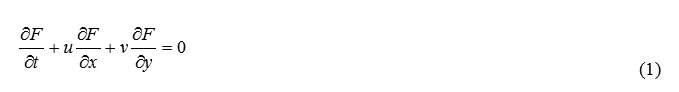
Where (u, v) are fluid velocities in the coordinate directions (x, y) or cylindrical coordinate directions (r, z) respectively. This equation states that F moves with the fluid.
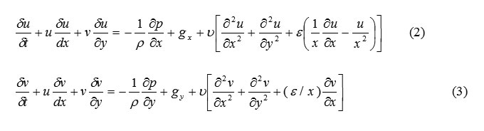
SOLA-VOF uses an Eulerian mesh of rectangular cells having variable sizes. δxi for the i th column and δyj for the j th row (Fig. 1). The fluid equations to be solved are the Navier-stocks equations:
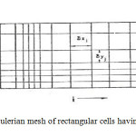 |
Fig1: An Eulerian mesh of rectangular cells having variable sizesClick here to View Figure |
The choice of coordinate system is governed by the value of ε, where ε=0 corresponds to Cartesian and ε=1 to cylindrical geometry. Body accelerations are denoted by (gx, gy) and ν is the coefficient of kinematic viscosity. Fluid density is denoted by ρ. For an incompressible fluid, the momentum equations, Eq. (2) and (3), must be supplemented with the incompressibility conditions:
The choice of coordinate system is governed by the value of ε, where ε=0 corresponds to Cartesian and ε=1 to cylindrical geometry. Body accelerations are denoted by (gx, gy) and ν is the coefficient of kinematic viscosity. Fluid density is denoted by ρ. For an incompressible fluid, the momentum equations, Eq. (2) and (3), must be supplemented with the incompressibility conditions
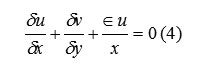
Sometimes, it is desirable to allow limited compressibility effects (e.g., acoustic waves), in which case eq. (4) must be replaced with
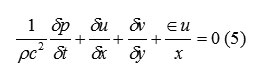
Where “c” is the adiabatic speed of sound in the fluid. Because Eq. (5) adds more flexibility with little additional complexity, it is incorporated as a standard feature in SOLA-VOF.
The procedure consists of three steps
- Momentum equation approximations to calculate the new velocities.
- Velocities computed from first step must satisfy the continuity equation.
- Update F.
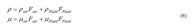
A solution may be obtained by the upper iterative process. It is used to calculate density and viscosity in a cell from averaging.
Simulation of bubble formation
In this investigation, the SOLA-VOF code was used to simulate the nano-bubble formation. In this code, it was used a variable grid to solve above equations using finite difference method. The geometry is shown schematically in Fig. 2. A cylindrical vessel with 4 μm diameter and 5 μm height is initially filled with 3 μm of liquid water. On the bottom there exists an orifice of diameter dor, from this orifice is injected constant air flow rate with velocity uor.
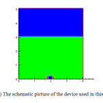 |
Fig2: The schematic picture of the device used in this study
|
Results and discussions
In this study, two cases were investigated. In the first case, hole diameter was about 250 nm and in the second case, it was 150 nm. The superficial velocity in the hole was 0.5 μm/s, 1 cm/s, 1.5 μ/s and 2 μ/s.
4-1) Effect of air flow rate on nano-bubble diameter
Tables (1) and (2) show the effect of air flow rate on nano-bubble diameter. If the effect of surface tension is neglected, the nano-bubble size is determined by the balance of Buoyancy, inertia and viscous forces for liquids with low viscosity. Accordingly, Davison (1960) presented the following equation to calculate the bubble diameter [15]
Table 1) Comparing bubble diameter (dor=250 nm)
|
2. |
1.5 |
1. |
0.5 |
UOR(μm/s) |
|
234 |
168 |
135 |
81 |
Db(VOF) nm |
|
138 |
123 |
104 |
79 |
Db(7) nm |
|
85 |
77 |
69 |
58 |
Db(8) nm |
Table 2) Comparing bubble diameter (dor=150 nm)
|
2. |
1.5 |
1. |
0.5 |
UOR(μm/s) |
|
111 |
99 |
81 |
60 |
Db(VOF) mm |
|
92 |
0.83 |
69 |
53 |
Db(7) mm |
|
73 |
68 |
61 |
51 |
Db(8) mm |

Here the units are based on SI system. Also Tribal used the following equation in his book to calculate the nano-bubble diameter for low gas flow rate (for liquids with a viscosity < 1000 cp) [4].
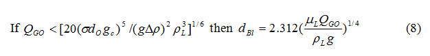
The purpose of the above equations, the purpose of the above equations is the comparison between the results of simulation and the results of equations (7) and (8), although these equations are approximate.
It should be noted that Tribal formulas can be used only in certain areas and it has not high performance range. The results of tables 1 and 2 show that nano-bubble diameter and its volume increase with increasing superficial velocity in the nozzle.In addition, the nano-bubble diameter calculated by the code is comparable with the nano-bubble diameter calculated from equations (7) and (8) and it is from an order. Therefore the results of this work are suitable and acceptable. Also it can be resulted that the nano-bubble diameter increases with increasing the orifice size.
4-2) Effect of air flow rate on the time of nano-bubble formation
Tables (3) and (4) show the effect of air flow rate on the time of nano-bubble formation. As illustrated in tables (3) and (4), the time of nano-bubble formation decreases with increasing superficial velocity in the nozzle. The time of nano-bubble formation is the time that nano-bubble release from nozzle. In other words, the time of nano-bubble formation decrease with increasing nano-bubble volume. Figure (3) shows bubble formation process for orifices with diameter 150 nm and speed 1.5 μm/s.
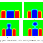 |
Fig3: Nano-bubble formation process in water (dor=150 nm, uor=1.5 μm/s) Click here to View Figure |
Table 3) Effect of superficial velocity on the time of bubble formation (dor=250 nm)
|
2. |
1.5 |
1. |
0.5 |
UOR(μm/s) |
|
0.07 |
0.074 |
0.078 |
0.1 |
tformation(s) |
Table 4) Effect of superficial velocity on the time of bubble formation (dor=150 nm)
|
2. |
1.5 |
1. |
0.5 |
UOR(μm/s) |
|
0.063 |
0.068 |
0.079 |
0.11 |
tformation(s) |
Conclusions
In this study, the nano-bubble formation process was simulated in a cylindrical container with an orifice submerged in water. Simulation was performed using SOLA-VOF numerical model.
In this process, two orifices with different diameters were used and air flow rate was assumed very low. Also it was understand that nano-bubble volume increase with increasing air flow rate and the time of nano-bubble formation decrease with increasing air flow rate. In addition, nano-bubble volume increase with increasing hole size in constant flow rate.
References
- Scott, T.; Banks, D.; Mishra, A. ApplBiosaf.,2006, 11(4), 188-196.
- Agarwal, A.; Ng, W.; Liu, Y. Chemosphere, 2011, 84 (9), 1175–1180
- Park, P.Y.; Tyler, A.L.;Nevers, N. Chem. Eng. Sci., 1997, 32, 907-916.
- Valencia, A.; Cordova, M.; Ortega, J. Int. Comm. Heat Mass Transfer,2002, 29, 821-830.
- Treybal, R.E. Mass Transfer Operation, Third Edition, 2003.
- Terasaka, K.;Tsuge, H. Chem. Eng. Sci., 1991, 46, 85-93.
- Terasaka, K.;Tsuge, H. Chem. Eng. Sci., 2001,56, 3237-3245.
- Yan, K.;Che, D.Int. J.Multiphase Flow, 2011, 37, 299-325.
- Chen, Y.; Mertz, R.;Kulenovic, R. Int. J. Multiphase Flow, 2009, 35, 66-77.
- Nichols, B.D.; Hirt,C.W.; Hotchkiss,R.S. Los Alamos National Scientific Laboratory, 1980, 119.
- Krishna, R.; van Baten, J.M. Int. Comm. Heat Mass Transfer,1999, 26, 965-974.
- Szewc, K.; Pozorski, J.; Minier,J. P. Int. J. Multiphase Flow,2013,50, 98-103.
- Zhang, W.; Tan, R.B.H. Chem. Eng. Sci., 2000, 55, 6243-6250.
- Sarnobat, S. U.; Rajput, S.;Bruns,D.;Depaoli, D.W.; Daw, C.S.; Nguyen, K. Chem. Eng. Sci., 2004, 59, 247-258.
- Davison, J.F.; Schuler, B.O.G. Trans.Instn.Chem. Engrs. 1960, 38, 335-342.
- Li, H. Z.;Mouline, Y.;Midoux, N. Chem. Eng. Sci., 2002, 57, 339-346.
- Kothe, D.; Rider,B; William,J. Los Alamos National Laboratory, 1995.

This work is licensed under a Creative Commons Attribution 4.0 International License.
![]()
A New Edition of Web of Science
Journal Impact Factor
2022: 0.5
Five Year: 0.8
Journal is Indexed in

Cabells Whitelist
![]()