Impact of Artisanal Gold Mining on Vegetation Cover and the Chemical and Physical Waters Quality
 , Saint Jean Patric Houebagnon Coulibaly2, Ahbeauriet Ahmed Ouattara1, Benjamin Kouassi Yao3
1Unité de formation et de recherche des sciences et technologies de l’Université Alassane Ouattara BP v18 Bouake 01
2Laboratoire de Télédétection et SIG, Centre Universitaire de Recherche et d’application en télédétection, Université Felix Houphouët-Boigny Abidjan, Côte d’Ivoire
3Nouvelles (LAPISEN Génie des procédés, Institut National Polytechnique Felix Houphouët-Boigny, Yamoussoukro, Côte d’Ivoire
Corresponding Author E-mail:horosebastien@yahoo.fr
Download this article as:
ABSTRACT:Illegal and artisanal gold mining has negative consequences in the Hambol region. Cadmium (Cd), with a contamination factor (CF) of 6.596, and mercury (Hg), with a contamination factor (CF) of 93.237, are the metals with very high levels of contamination. Furthermore, the enrichment factor (EF) for cadmium (36.644) which falls within the range of 20 to 40 indicates contamination approaching extreme levels. As for mercury, it exhibits extreme contamination, as indicated by an EF of 149.18, which is well above 40. Statistical analysis supported by the mercury geoaccumulation index showed that this metal originates from an anthropogenic source. However, the Pollutant Load Index (PLI) ˂ 1 indicates that metal contamination has not been confirmed, even though the mercury and cadmium values remain higher than those of the continental crust (VCC). Land-use analysis showed that this gold panning activity is impacting vegetation cover, with nearly 692.71 ha already occupied.
KEYWORDS:Artisanal Gold Mining; Hambol Region; Illegal Gold Mining; Land Use
Introduction
Recent decades have been marked by an explosion in mining activity across many countries around the world. Africa, with an economy heavily dependent on agricultural production, faces economic challenges due to fluctuations in agricultural commodity prices. However, while some African countries have managed to sustain their economies through industrialization, the same cannot be said for those in sub-Saharan Africa particularly Côte d’Ivoire, where agriculture remains the backbone of the economy (Soro, 2011; Akpo et al., 2022). Consequently, rural populations who depend solely on agriculture for their livelihoods are forced to explore other sources of income, such as small-scale gold mining. This activity, which generates significant financial resources, contributes approximately 1% to GDP (Yapi et al., 2014; Akpo et al., 2022). In fact, according to a report by the newspaper Le Monde Afrique published on July 6, 2021, more than 500,000 people are involved in this activity. It has become an integral part of the local economy (Kouassi and Yapo, 2021; Kone et al., 2024). Despite the benefits associated with this activity, it remains a major problem when it is not properly regulated and controlled. Illegal gold mining, also known as clandestine mining, causes more harm than good to rural communities. Whether industrial or artisanal, gold panning results in the loss of arable land (Akpo et al., 2022). In addition to actively contributing to the destruction of arable land, illegal gold panning is one of the causes of pollution in water sources near the sites where it is practiced. Camps are set up to house the gold panners. All these gold miners defecate in the open, and some use motorized equipment. Furthermore, washing the tailings to extract gold causes the water to become highly turbid. Today, this activity affects every community. Decisions to implement solutions are being made, but remain insufficient to stop this activity. Beyond the study area, this issue persists in many localities across sub-Saharan Africa. However, studies generally focus only on known gold mining sites and overlook small villages. This is the case for sites located between the villages of Pétionara, Tiengala, and Serigbokaha. These villages, located in the Hambol region, have all lost their economic lifeblood to small-scale gold mining. 80 % of the youth in these villages are involved in this activity. However, certain chemicals, such as mercury, are sometimes used when washing the ore. Given the scale of this activity, which is on the verge of causing a famine and a water crisis, a survey is essential to limit the damage. With this in mind, this study was initiated to examine the physical and chemical characteristics of the water at a site located northeast of Niakara and east of Pétionara. The study also highlights the impact on land use.
Materials and Methods
Materials
Geographic Location
The artisanal gold mining site covered by this study is located in the Hambol region, specifically in the Niakara Department, east of Comoé National Park. The backwaters and channels sampled were selected within this same department, which contains several clandestine artisanal gold mining sites (Figure 1).
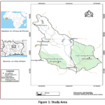 |
Figure 1: Study Area Click here to View Figure |
Land Use in the Pétionara Watershed
The goal was to develop an integrated method combining Sentinel-1, Sentinel-2, and Random Forest to map land use and automatically detect artisanal gold mining sites.
Satellite Data
The characteristics of the satellite data used are listed in Table 1.
Table 1: Characteristics of the images used for land cover analysis
|
Sentinel-2 |
Sentinel-1 | |
| Bande | Resolution |
VV |
|
B2 |
10 m | VH |
| B3 | 10 m |
VV−VH |
|
B4 |
10 m | VV/VH |
| B8 | 10 m |
DEM |
|
B11 |
20 m | Copernicus DEM 30 m |
| B12 | 20 m |
Elevation |
Water Samples
The water samples were collected from several sites. First, four sampling points were identified along the Tchonrhon River. The first point was selected upstream of the gold panning site, the second at the washing site, the third in the dug pits, and the fourth downstream of the gold panners’ site. Next, the samples that were not analyzed on site were refrigerated and transported to the laboratory. Finally, the samples were analyzed in the laboratory according to the protocols provided by Rodier et al. (2009).
Analytical Equipment
The equipment used consisted of portable devices, some of which were used to measure certain parameters in situ and others in the laboratory. For in situ analyses, a portable, microprocessor-equipped multiparameter probe (pH/Cond 340i set b, WTW, England) was used. Using this device, parameters such as pH, temperature, electrical conductivity, total dissolved solids (TDS), salinity, and dissolved oxygen were measured. The remaining chemical parameters were determined using a DR 2800 multifunction spectrophotometer (F HACH, USA). Each parameter was measured using the corresponding reagent kit. A wavelength scan corresponding to each parameter was performed. Thus, the concentration of each species was assessed in the water. Samples consisting of soil sediments and water were collected exclusively on-site for soil samples and from the nearby river and depressions on the site for water samples. Soil sediment samples were collected using a Van Veen sampler at the river and a polyethylene spatula along the riverbank, then placed in glass bottles that had been previously washed and rinsed with deionized water. Water samples were collected using glass bottles that had been washed and rinsed with deionized water. Metals, on the other hand, were analyzed using X-ray fluorescence. This technique is widely used for the analysis of trace elements in geological materials, soils, and sludge prepared in the form of pressed pellets. The SPECTRO XEPOS (AMETEK model, France) is a benchtop XRF spectrometer designed for multi-element analysis to identify and quantify the chemical elements present in a sample.
Methods
Land-Use Mapping Method
The methodology adopted combines Sentinel-2 optical data, Sentinel-1 radar data, and a Random Forest supervised classification algorithm. This data set was used to map land cover and detect artisanal gold mining sites (Belgiu & Drăguț, 2016; Maxwell et al., 2018) (Phiri, D. et al., 2020). First, the Sentinel-2 images were preprocessed to remove pixels affected by clouds and their shadows. The Scene Classification Layer (SCL) was used to perform this operation. A median composite for January 2026 was then generated to reduce the effects of residual atmospheric conditions and outlier observations (Drusch et al., 2012). Next, Sentinel-1 images were selected based on VV and VH polarizations as well as the IW acquisition mode. Finally, speckle noise reduction was performed using spatial filtering (Torres et al., 2012) (Venter, 2021) (Veloso et al., 2017). A median composite was then calculated to obtain a representative radar image for January 2026.
Calculation of Spectral Indices
Several indices were calculated using Sentinel-2 data. These indices are used to characterize the different types of land cover. Radar data were then used to derive additional variables describing the backscattering properties of surfaces. Textural measures based on the gray-level co-occurrence matrix (GLCM) were also extracted to better characterize the spatial heterogeneity of gold mining areas (Haralick et al., 1973).
Data Fusion
All spectral bands, indices, radar variables, textures, and topographic variables were then fused into a single multidimensional image. This image constitutes the set of explanatory variables used for classification.
Training Data
This data was compiled from training polygons. It represents the various land-use classes identified in very high-resolution images and validated through visual interpretation. The samples were then randomly divided into two sets, with 70% used for model training and 30% reserved for independent validation.
Classification
Classification was performed using the Random Forest algorithm. This algorithm is known for its robustness with multidimensional data and its ability to limit overfitting (Zhang et al. 2019). The model was then evaluated using a confusion matrix to calculate overall accuracy, the Kappa coefficient, receiver operating characteristic (ROC) curves, and the F1 score for each class.
Variables Used
All explanatory variables used to train the Random Forest model are derived from Sentinel-2 optical data, Sentinel-1 radar data, spectral indices, radar textures, and topographic variables (Figure 2). The methodology adopted combines Sentinel-2 optical data, Sentinel-1 radar data, and a supervised Random Forest classification algorithm. The goal is to map land cover and detect artisanal gold mining sites (Belgiu & Drăguț, 2016; Maxwell et al., 2018) (Phiri, D. et al., 2020). Six main classes were identified: forests, savannas, croplands, bare ground, water bodies, and artisanal gold mining areas. Classification accuracy was assessed using independent validation based on reference samples
Table 2: Variable characteristics
|
Category |
Variables |
|
Optical bands (Sentinel-2) |
B2 (Blue), B3 (Green), B4 (Red), B8 (Near-Infrared), B11 (SWIR1), B12 (SWIR2) |
| Spectral indices |
NDVI, BSI, MNDWI, NDBI, NDRE, SAVI, NDTI, TURBIDITY, NBR2 |
|
Radar variables (Sentinel-1) |
VV, VH, VV−VH, VV/VH |
| GLCM texture |
VV Contrast, VV Entropy, VV Homogeneity (IDM), VH Contrast, VH Entropy, VH Homogeneity (IDM) |
|
Topographic variables |
Elevation (Copernicus DEM) |
Artisanal Method of Gold Detection
Artisanal gold panning remains widespread in various areas of Côte d’Ivoire. Photo 2 shows how gold is extracted using artisanal methods after stripping away the topsoil. The direct and visible impact of this artisanal method is the change in the color of the surrounding surface waters. Photo 3 (Yassin Ciyow, 2021).
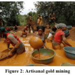 |
Figure 2: Artisanal gold mining Click here to View Figure |
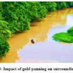 |
Figure 3: Impact of gold panning on surrounding rivers Click here to View Figure |
Measurement of Chemical Parameters
The chemical and physical parameters at the site were measured by immersing the probe of the portable multiparameter meter into the samples in situ. The readings were taken directly from the device’s screen to provide quantitative values for each chemical species.
The other chemical parameters were determined using their respective reagents in the DR 2800 multifunction spectrophotometer. Each parameter was measured at a specific wavelength unique to that parameter. Thus, each parameter was detected at its respective wavelength. The standards used are listed in Table 3.
Table 3: Methods for Analyzing Chemical and Physical Parameters
|
Physical and Chemical Properties of Water |
Equipment | Standards |
| Temperature (°C) | Portable Multi-Parameter Sensor, pH/Cond 340i Set B |
AFNOR NF T90-008 |
|
Hydrogen Ion Concentration (pH) |
AFNOR NF ISO 10523 | |
| Electrical Conductivity (EC) |
AFNOR NF EN 27888 |
|
|
Total Dissolved Solids (TDS) |
||
|
Salinity (‰) |
||
|
Dissolved Oxygen (DO) |
AFNOR NF EN 25813 | |
| Nitrates (NO3–) | DR 2800 |
AFNOR ISO 7890-3 |
|
Nitrites (NO2–) |
AFNOR ISO 7890-3 | |
| Ammonium (NH4+) |
AFNOR ISO 6778 |
|
|
Orthophosphate (PO43-) |
AFNOR NF T90-023 | |
| Total Phosphorus |
AFNOR ISO 6878 |
|
|
Sulfates (SO42-) |
AFNOR (T90-040) | |
| Biochemical Oxygen Demand (BOD5) |
AFNOR NF EN 1899 |
|
Trace Element Detection
The sample pellets were analyzed in the XRF system at an X-ray tube voltage of 34.80 kV and a current of 1 mA. A low-power X-ray tube was used as the radiation source for the simultaneous analysis of elements ranging from sodium to uranium. Each complete analysis took approximately 15 minutes. The measurements were performed using a SPECTRO XEPOS equipped with a 50-W X-ray tube with a Pd end window. Forced-air cooling was used for a high-resolution SDD, called VITUS, and an 8-position target changer comprising a Bragg monochromatic (HOPG) and a Barkla polarizer. The resolution of the VITUS detector was set to 149 eV (Mn Kα) with an input count rate of 100,000 cps. The chamber was purged with helium N 60 (99.9999%) prior to all measurements. Furthermore, the concentration of each element was determined using software (X-LabPro). The results were processed using Spectraplus software. Metal concentrations were expressed in mg/kg of dry weight. The concentrations of the 10 trace metals namely Zn, Cr, Ni, Pb, Cu, Cd, V, Mn, Fe, Al, and As were determined (Oura et al., 2022).
Analysis of Soil Sediments
First, the collected sediments were dried at room temperature (approximately 23°C) for several days until they reached a constant weight. Next, 20 grams (20 g) of the samples were sieved to remove gravel and coarse debris using a series of sieves with varying mesh sizes: 2 mm, 1 mm, 500 μm, and 250 μm. Subsequently, a vibratory ball mill (RETSCH GmbH, Type MM400; 42781 Haan, Germany) was used to grind and homogenize an aliquot of the sample after sieving. The homogenized ground material was sieved again to obtain an average grain size of approximately 60 μm. Finally, four grams (4 g) of the ground sample material were taken and mixed with 1 g of binder (Fluxana BM-0002-1-CEROX). The mixture was then compressed into an aluminum cartridge using a 15-metric-ton press (Specac; Atlas TM manual 15Ton (Oura et al., 2022).
Determination of Indices for Assessing Pollution and Its Source
The extent of anthropogenic impacts on sediment quality was assessed by calculating three (3) parameters: the enrichment factor (EF), the contamination factor (CF), and the pollutant load index (PLI). The calculation method used is that applied by Feng et al. (2011) and Oura et al. (2021) for CF and PLI (Equations 1 and 2). As for the enrichment factor (EF), the calculation method used is that of Sutherland et al. (2004) and Oura et al. (2021) (Equation 3). Since aluminum is a good tracer and a major constituent of clay minerals, it was considered the reference metal for measuring the concentrations of other metals (Oura et al., 2021). Given the high concentration of aluminum in the sediments, its artificial enrichment is unlikely. For this reason, Karaouzas et al. (2021) and Oura et al. (2021) selected it as an index for assessing anthropogenic influences on the sediments.
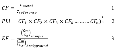
For Equation 3
Where Cm = concentration of the metal in the sediments and Cx = concentration of aluminum (Al) in the sediments.
The results were interpreted with reference to Sutherland et al. (2004). According to these authors, if: EF < 2: minimal contamination; 2 < EF < 5: moderate contamination; 5 < EF < 20: significant contamination; 20 < EF < 40: high contamination; and EF > 40: extreme contamination. For the quantitative assessment, the CF factor was taken into account. Thus, if CF < 1, this indicates low contamination; 1 < CF < 3 corresponds to moderate contamination; 3 < CF < 6 corresponds to considerable contamination; and CF > 6 corresponds to very high contamination (Oura et al., 2021). Based on CF, Thomson (1980) introduced the pollution load index. If PLI > 1, metal pollution is confirmed; otherwise, if PLI ≤ 1, metal pollution remains uncertain. Finally, the geoaccumulation index proposed by Muller [28] and Kim et al. (2018) was calculated using the following equations:
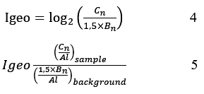
Where Cn corresponds to the measured concentration of the metal (n) in the sediments,
Bn to the geochemical background concentration of the metal (n), and 1.5 to the correction factor introduced to minimize any effects of variations in background values that could be attributed to variations in sediment lithology (Xu et al., 2020) The results were interpreted taking into account the ranges listed in the table (Barbieri, Maurizio, 2016; Kim et al., 2018).
Table 4: Igeo Categories
|
class |
value | Soil dust quality |
| 0 | Igeo ≤ 0 |
Uncontaminated |
|
1 |
0 ≤ Igeo ≤ 1 | Uncontaminated to moderately contaminated |
| 2 | 1˂ Igeo ≤ 2 |
Moderately contaminated |
|
3 |
2˂ Igeo ≤ 3 | Moderately to heavily contaminated |
| 4 | 3˂ Igeo ≤ 4 |
Heavily contaminated |
|
5 |
4˂ Igeo ≤ 5 | Heavily to extremely contaminated |
| 6 | Igeo > 5 |
Extremely contaminated |
Statistical Analysis
The statistical analysis was performed using XLSTAT software (version 2017). This analysis identified the group of parameters responsible for diffuse pollution as well as the anthropogenic source of copper. A difference was considered significant at p < 0.05. This analysis also revealed correlations between physical and chemical parameters and heavy metals.
Results and Discussion
Classification Performance
Supervised classification based on the Random Forest algorithm made it possible to distinguish six land-use classes: forest, savanna, cropland, bare soil, water, and artisanal gold mining sites. Independent validation produced a confusion matrix from which the overall accuracy, Kappa coefficient, and F1 score were calculated. With an overall accuracy of 96%, the model correctly classifies the vast majority of pixels. The Kappa coefficient, equal to 0.95, confirms the model’s robustness and the reliability of its predictions.
Confusion Matrix
The model’s overall performance is good. The values on the diagonal (in bold) are very high (Table 5). This confirms the good accuracy (0.96) and Kappa (0.95) scores. Most pixels are correctly classified. The “gold panning” class is well classified (887 pixels), but a few pixels are misclassified as water (10 pixels) and forest (9 pixels). This could be due to the presence of puddles and vegetation at the mining sites.
Table 5: Confusion matrix
|
Actual Classes \ Predicted |
Crops | Forests | Savannas | Water | Bare ground | Orpaillage | Total Predicted |
| Crops | 2835 | 25 | 24 | 0 | 0 | 0 |
2884 |
|
Forests |
63 | 1039 | 75 | 5 | 0 | 0 | 1182 |
| Savannas | 78 | 23 | 1523 | 0 | 0 | 0 |
1624 |
|
Water |
0 | 10 | 0 | 1787 | 0 | 1 | 1798 |
| Bare Soil | 9 | 1 | 0 | 0 | 8 | 1 |
19 |
|
Gold Panning |
1 | 9 | 0 | 10 | 0 | 887 | 907 |
| Total Predicted | 2986 | 1107 | 1622 | 1802 | 8 | 889 |
8414 |
Land-Use Mapping
Savanna and forest cover 72% of the area, confirming that the dominant vegetation type is wooded savanna. The categories “Bare and Built-up Land” (4.16%) and “Gold Panning” (3.99%) account for similar proportions, reflecting significant pressure from gold panning activities. The presence of this activity calls for increased monitoring, as it can cause soil degradation and watercourse alteration.
Table 6: Area Occupied by Different Land-Use Categories
|
Class |
Surface (ha) |
% |
|
Forest |
4991.05 | 28.72 |
| Savanna | 7593.38 |
43.70 |
|
Cultivated Land |
3376.52 | 19.43 |
| Bare Ground | 722.91 |
4.16 |
|
Water |
0.682 | 0.0039 |
| Gold Panning | 692.71 |
3.99 |
Spatial Distribution of Mining Sites
Artisanal gold mining sites are mainly concentrated along the river system around the Kiohan River, northeast of Pétionara and southeast of Angolokaha (Figure 4). Mining activities are also observed along the river to the west of the Kipelekaha settlement. This distribution illustrates the dependence of artisanal mining operations on alluvial gold deposits.
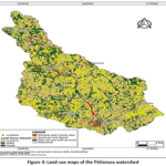 |
Figure 4: Land-use maps of the Pétionara watershed Click here to View Figure |
Determination of the CF, EF, Igeo, and PLI indices for sediments
Continental crust values (VCC) are considered background values (Gao and Chen, 2012; Hu et al., 2013; Rudnick et al., 2003; Oura et al., 2021). By comparing the average trace metal concentrations in the sediments with those of the continental crust, we can already identify toxic metals in the study area (Table 7). The table shows that metals such as iron (Fe), arsenic (As), and mercury (Hg) have higher average concentrations than those in the continental crust. According to Hu et al. (2013) and Oura et al. (2021), these metals (Fe, As, and Hg) are toxic to the areas surrounding artisanal gold mining sites. The high concentration of mercury in the baffon sediments and the areas surrounding the artisanal gold mining sites is likely the result of runoff and seepage (Hue et al., 2020; Bohbo et al., 2017; Chevrillon-Guibert et al., 2019; Keita, 2017; Tahirou et al., 2024). Indeed, during the rainy season, the river overflows and floods the surrounding alluvial fans. According to the CF values in the table, metals such as Al, Zn, Cr, Ni, Pb, Cu, Fe, and As cause only low levels of contamination in the sediments of the study area, as their CF values are less than 1 (Oural et al., 2021). However, cadmium (Cd) and mercury (Hg), with CF values of 6.596 and 93.237, respectively both greater than 6 exhibit very high levels of contamination. In addition to CF values, EF values were used to assess the pollution levels of each metal. Thus, the sediments exhibit minimal contamination for the metals Al, Zn, Cr, Ni, Pb, Cu, Fe, and As. As for Cd, with an EF ranging from 20 to 40, it constitutes a high level of contamination in the sediments. Mercury, with an EF of 149.18, remains the most heavily contaminated metal. Once again, the geoaccumulation indices show that none of the metals are contaminating the sediments studied. However, cadmium, with a GeoAccumulation Index (Igeo) of 3.078 which falls between 3 and 4 indicates high contamination. Copper, on the other hand, tends toward extreme contamination of the sediments. Indeed, its geoaccumulation index of 4.823 falls within the range of 4 to 5 (Barbieri, Maurizio, 2016; Kim et al., 2018). Given the GeoAccumulation Indices (Igeo) for cadmium and mercury, these metals may originate from anthropogenic activities such as gold panning. According to the Pollutant Load Index (PLI), which is 0.236 ˂ 1, metal pollution is uncertain (Oural et al., 2021).
Table 7: Trace metals and their factors and indices
|
Locations |
Al | Zn | Cr | Ni | Pb | Cu | Cd | Fe | As | Hg |
| Bafon 1 | 185 | 18.25 | 83.42 | 11.52 | 4.65 | 7.33 | 3.22 | 230.17 | 2.93 |
8.83 |
|
Bafon 2 |
188.5 | 16.92 | 14.82 | 10.75 | 3.35 | 5.62 | 3.80 | 218.33 | 2.13 | 8.23 |
| Bafon 3 | 197.5 | 14.22 | 33.68 | 10.40 | 1.63 | 5.88 | 3.38 | 232 | 2.75 |
12.45 |
|
Bafon 4 |
169.5 | 8.57 | 54.6 | 13.68 | 3.43 | 5.07 | 3.37 | 229.83 | 2.68 | 10.28 |
| Bafon 5 | 187 | 6.77 | 57.92 | 9.77 | 3.40 | 5.43 | 3.60 | 279.98 | 2.20 |
8.22 |
|
Champ 1 |
141 | 3.72 | 39.6 | 7.78 | 1.43 | 3.13 | 3.78 | 222.33 | 3.10 | 12.41 |
| Champ 2 | 130 | 4.20 | 14.92 | 4.20 | 1.70 | 4.20 | 2.67 | 222.82 | 5.22 |
2.62 |
|
Champ 3 |
152.5 | 6,55 | 10.42 | 2.42 | 1.12 | 4.92 | 3.88 | 230 | 6.43 | 2.83 |
| Champ 4 | 163.75 | 4.92 | 57.65 | 4.67 | 1.40 | 3.65 | 2.33 | 204.33 | 4.25 |
4.85 |
|
Champ 5 |
129.25 | 4.25 | 32.97 | 4.7 | 1.30 | 4.55 | 2.95 | 210.67 | 4.47 | 3.87 |
| Average | 164.4 | 8.837 | 40 | 7.989 | 2.341 | 4.98 | 3.298 | 228.05 | 3.62 |
7.46 |
|
UCC |
83 100 | 67 | 92 | 47 | 17 | 28 | 0,09 | 39 200 | 5 | 0,05 |
| VRM | 8-8.13% | 50 -70 mg/Kg | 35-100 | 20-47 | 10 à 15 | 25-28 | 0,1-0,2 | 3,5-5,63 | 1,5-5 |
0,02 |
|
VDS |
80000 | 50 -70 mg/Kg | 50 | 15-40 | 10 à 20 | 15-30 | 0,1-0,5 | 50000 | 5 à 15 | |
| CF | 0.002 | 0.126 | 0.8 | 0.199 | 0.117 | 0.166 | 6.596 | 0.004 | 0.241 |
93.237 |
|
EF |
0.002 | 0.132 | 0.435 | 0.169 | 0.138 | 0.178 | 36.644 | 0.006 | 0.723 | 149.18 |
| Igeo2 | -6.816 | -2.832 | -0.965 | -2.016 | -2.551 | -2.712 | 2.397 | 3.078 | -0.219 |
4.823 |
|
PLI= 0.236 |
||||||||||
Statistical Analysis of Physical and Chemical Parameters and Metals
Selection of Factors
Factor analysis of the chemical and physical data from the samples led to the selection of three factors (F1, F2, and F3) (Table 8), based on their respective eigenvalues of 6.018, 2.872, and 1.109. Indeed, a factor is considered significant if its eigenvalue is greater than or equal to 1 (Koné et al., 2022; Kouakou et al., 20216). In addition, the three factors collectively explain 100% of the total variance. Furthermore, the sum of the eigenvalues is equal to the number of initial variables, which is 10. The parameters are correlated with the different factors F1, F2, and F3, accounting for 60.2%, 28.7%, and 11.1% of the variance, respectively (Table 1). Factor F1, which involves organic and nitrogen pollution or mineralization, encompasses nearly all of the organic and nutrient contamination parameters. In fact, strong negative correlations for NO₂⁻ (r = −0.94), NO₃⁻ (r = −0.93), NT (r = −0.90), NH₄⁺ (r = −0.84), BOD5 (r = -0.83), and PO43- (r = -0.69) were observed with F1. Unlike the other parameters, pH (r = 0.95) shows a strong positive correlation. Given the negative correlations, this factor is associated with waters that are heavily loaded with nitrogen, organic matter (BOD5), and phosphate.
These pollutants cause contamination that may originate from domestic sources, agriculture, or wastewater treatment (sewage discharge, fertilizer runoff), resulting in water with higher mineral content and a higher pH. Factor 1 can be considered the primary driver of water quality degradation based on the analyzed parameters. It alone encompasses all the classic parameters of eutrophication and organic pollution (nitrogen in its three forms, phosphate, and BOD5). Yang et al. (2020) made a similar observation in their study on the use of PCA to determine spatiotemporal changes in surface water. As for factor F2, which accounts for 28.7% of the variance, it is a factor related to temperature and particulate load. Temperature is the dominant parameter of this factor (r = 0.96). However, factor F2 is negatively correlated with turbidity (r = -0.77) and with orthophosphates (r = -0.72). Given the parameters with which this factor is correlated, it likely reflects a seasonal effect. High temperatures would indicate a dry season accompanied by reduced turbidity and phosphate inputs. In contrast to the dry period, rainfall accompanied by runoff increases turbidity and phosphorus inputs. This factor therefore reflects hydro-climatic variation rather than a specific source of pollution. This correlation of the parameters (T, turbidity, and orthophosphates) with factor 2 corroborates the study by Yang et al. (2020) on watersheds.
Like factors 1 and 2, factor 3, which accounts for 11.1% of the variance, is specific to sulfate (r = -0.78). The isolation of sulfates into a distinct factor suggests a source separate from the first two axes. This source could potentially be linked to the oxidation of certain sulfide minerals (acid mine drainage) or to rock of geological origin that has undergone specific anthropogenic impacts related to gold panning.
In fact, the weathering of sulfides associated with gold deposits can lead to significant inputs of sulfates into surface waters. This is supported by Gomes & Valente (2024), who demonstrated that high sulfate concentrations, followed by a marked decrease in pH, result from water affected by acid mine drainage stemming from the oxidation of sulfide minerals (Gomes & Valente, 2024).
Table 8: Selection of factors based on eigenvalues of physical and chemical parameters
|
Variables |
Fact. 1 | Fact. 2 |
Fact. 3 |
|
N (mg/L)) |
-0.902 | -0.400 | -0.159 |
| NO2– (mg/L)) | -0.942 | 0.167 |
-0.289 |
|
NO3– (mg/L) |
-0.932 | 0.082 | -0.351 |
| NH4+ (mg/L) | -0.843 | 0.514 |
-0.158 |
|
Turbidité (NTU) |
-0.523 | -0.767 | 0.370 |
| PO43- (mg/L) | -0.689 | -0.721 |
0.063 |
|
SO42-(mg/L) |
0.584 | -0.207 | -0.847 |
| DBO5 (mg/L) | -0.827 | 0.491 |
0.275 |
|
T (°C) |
0.235 | 0.962 | 0.137 |
| pH | 0.952 | -0.306 |
0.013 |
|
Equity |
6.019 | 2.872 | 1.109 |
| % of Total Variance | 60.186 | 28.722 |
11.091 |
|
Cumulative Equity |
6.019 | 8.891 | 10 |
| Cumulative % | 60.186 | 88.909 |
100 |
Analysis of Correlation Matrices between Parameters
The correlation tables in Table 9, associated with the correlation circles, reveal three clusters. One of the clusters, identified as the nitrogen and organic pollution cluster, shows several correlations (Figure 5). Within this cluster, NO₂⁻ and NO₃⁻ are strongly correlated (r = 0.99). These two parameters are also correlated with ammonium (NH₄⁺), with correlations of r = 0.93 and r = 0.88, respectively. As for BOD₅, correlations of r = 0.78 and r = 0.71 are observed with NO₂⁻ and NO₃⁻, respectively. The strong correlations observed between nitrogen compounds and organic matter corroborate the findings of Yang et al. (2020). Indeed, according to these authors, when nitrogen compounds and organic matter change in tandem, this suggests pollution from agricultural runoff or wastewater. The second cluster observed in the correlation table of physical and chemical water parameters is that of turbidity and phosphates. It appears that turbidity and phosphates are very strongly correlated (r = 0.94), and both have a negative correlation with temperature (r = -0.81 and -0.85). Unlike the other factors, pH is strongly and negatively correlated with all pollution indicator parameters, such as NH₄⁺ (r = -0.96), NO₂⁻ (r = -0.95), BOD₅ (r = -0.93), NO₃⁻ (r = -0.92), and NT (r = -0.74) . Given that the higher the concentration of nitrogen and organic matter in the water, the more the pH tends to decrease, the pH effect observed in this study is consistent. The distinct behavior of sulfates at factor 3 is confirmed by observations of generally negative correlations with indicators of organic pollution (r = -0.80 with BOD5). According to Esdaile & Chalker (2018), this type of behavior indicates a source of mining-related pollution linked to the fragmentation of a geological structure.
Table 9: Correlation between chemical and physical parameters
|
Variables |
NT | NO2– (mg/L)) | NO3– (mg/L) | NH4+ (mg/L) | Turbidité (NTU) | PO43- (mg/L) | SO42-(mg/L) | DBO5 (mg/L) | T (°C) | pH |
| NT | 1 | |||||||||
|
NO2– |
0.83 |
1 |
||||||||
|
NO3– |
0.86 | 0.99 |
1 |
|||||||
|
NH4+ |
0.58 | 0.93 | 0.88 |
1 |
||||||
|
Turbidity |
0.72 | 0.26 | 0.29 | -0.01 |
1 |
|||||
|
PO43- |
0.91 | 0.51 | 0.56 | 0.20 | 0.94 |
1 |
||||
|
SO42- |
-0.32 | -0.35 | -0.28 | -0.47 | -0.44 | -0.30 |
1 |
|||
|
DBO5 |
0.50 | 0.78 | 0.71 | 0.90 | 0.16 | 0.23 | -0.80 | 1 | ||
| T | -0.61 | -0.10 | -0.18 | 0.27 | -0.81 | -0.85 | -0.17 | 0.31 |
1 |
|
|
pH |
-0 ?74 | -0.95 | -0.92 | -0.96 | -0.25 | -0.43 | 0.6& | -0.93 | -0.07 |
1 |
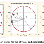 |
Figure 5: Correlation circles for the physical and chemical parameters of water Click here to View Figure |
Selection of factors for the statistical analysis of metals in water
Factors F1, F2, and F3, with respective eigenvalues of 5.302955, 3.071839, and 1.625205 all of which are greater than 1 are considered valid, as stipulated by the researchers Kaiser (1960), Kouakou et al. (2016), and Koné et al. (2022) (Table 10). In addition, their variances are 53.02955, 30.71839, and 16.25205, which together total 100%. Factor F1 is correlated with the metals As (r = -0.93), Cr (r = -0.91), Zn (r = -0.87), Pb (r = -0.84), Cu (r = -0.79), Ni (r = -0.71), and Cd (r = -0.67). Given the metals correlated with factor F1, this is likely to be diffuse pollution linked to mining residues and tailings, as well as to the erosion of disturbed soils. This finding is consistent with the work of Barde et al. (2024) conducted at other West African gold panning sites. Indeed, these authors observed a close association between Pb, Cd, Zn, and As originating from a common source linked to artisanal mining (Barde et al., 2024). The fact that mercury stands alone, showing only a weak correlation with the other metals, is telling. Furthermore, mercury stands out as the primary indicator of contamination linked to gold panning. In short, mercury is considered a tracer of amalgamation. Its geochemical behavior is generally largely independent of other trace metals of mineral origin (Esdaile & Chalker, 2018). This independence has, however, been reported in soils from gold mining sites in West Africa by Fagbenro et al. (2021). Like mercury, arsenic differs from the main polymetallic assemblage (Fagbenro et al., 2021).
Table 10: Selection of factors based on the eigenvalues of the metals
|
Variables |
Fact. 1 | Fact. 2 |
Fact. 3 |
|
Al (mg/kg) |
-0.291 | -0.931 | 0.221 |
| Zn (mg/kg) | -0.867 | 0.497 |
-0.045 |
|
Cr (µg/kg) |
-0.907 | 0.288 | 0.305 |
| Ni (mg/kg) | -0.714 | 0.662 |
-0.228 |
|
Pb (µg/kg) |
-0.844 | 0.320 | -0.429 |
| Cu (mg/kg) | -0.786 | -0.504 |
-0.358 |
|
Cd (mg/kg) |
-0.675 | -0.608 | -0.418 |
| Fe (mg/kg) | -0.540 | -0.837 |
0.082 |
|
As (mg/kg) |
-0.925 | 0.085 | 0.369 |
| Hg | -0.448 | 0.035 |
0.893 |
|
Equity |
5.303 | 3.072 | 1.625 |
| % of Total Variance | 53.029 | 30.718 |
16.252 |
|
Cumulative Equity |
5.303 | 8.375 | 10.000 |
| Cumulative % | 53.029 | 83.748 |
100.000 |
Correlation Study of Metals
Just like the correlation matrix for physical and chemical parameters, the correlation matrix for metals confirms and refines the three-factor structure (Table 11) and (Figure 6). A group comprising metals such as Zn, Ni, Cr, and Pb is strongly intercorrelated (Zn-Ni r = 0.96; Zn-Cr r = 0.91; Zn-Pb r = 0.91; Ni-Pb r = 0.91). In addition to these, arsenic joins this group, showing strong correlations with Cr (r = 0.98) and Zn (r = 0.83). This cluster points to a common source of pollution for these five elements, which is diffuse mining activity. One example illustrating the impact of gold panning on surface waters is the presence of iron and aluminum, which form a geogenic group. Indeed, Al and Fe are highly correlated (r = 0.95), as are Cu and Cd (r = 0.99). Just like cadmium (Cd) and copper (Cu), Fe (Fe-Cu r = 0.82; Fe-Cd r = 0.84) is also positively correlated. This Al-Fe-Cu-Cd cluster could suggest that Cu and Cd exhibit geochemical behavior more characteristic of the clay-iron fraction than of diffuse mining pollution. The fact that mercury stands apart, with a correlation of r = 0.75 with arsenic, indicates that it originates from a specific, point source of pollution.
Table 11: Correlation among the various metals
|
Variables |
Al | Zn | Cr | Ni | Pb | Cu | Cd | Fe | As | Hg |
| Al | 1 |
|
||||||||
|
Zn |
-0.22 | 1 | ||||||||
| Cr | 0.06 | 0.91 | 1 |
|
||||||
|
Ni |
-0.46 | 0.96 | 0.77 | 1 | ||||||
| Pb | -0.15 | 0.91 | 0.73 | 0.91 | 1 |
|
||||
|
Cu |
0.62 | 0.45 | 0.46 | 0.31 | 0.65 | 1 | ||||
| Cd | 0.67 | 0.30 | 0.31 | 0.17 | 0.55 | 0.99 |
1 |
|||
|
Fe |
0.95 | 0.05 | 0.27 | -0.19 | 0.15 | 0.82 | 0.84 | 1 | ||
| As | 0.27 | 0.83 | 0.98 | 0.63 | 0.65 | 0.55 | 0.42 | 0.46 |
1 |
|
|
Hg |
0.29 | 0.36 | 0.69 | 0.14 | 0.01 | 0.01 | -0.09 | 0.28 | 0.75 |
1 |
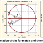 |
Figure 6: Correlation circles for metals and chemicals in water Click here to View Figure |
Conclusion
Artisanal gold mining remains a threat to aquatic life and to the communities that practice it. In addition to negatively impacting vegetation cover, gold mining causes both metallic and chemical pollution. Given the high CF, Igeo, and EF indices for mercury and cadmium, illegal and artisanal gold mining must be halted in this part of the Hambol region to ensure a future for coming generations. Effective awareness-raising efforts, accompanied by rigorous measures, must be implemented to mitigate the disaster that this situation could cause if the activity continues. At the very least, the government must better regulate this activity in the region and restrict the areas where gold mining is permitted.
Funding Sources
The author(s) received no financial support for the research, authorship, and/or publication of this article.
Conflict of Interest
The author(s) do not have any conflict of interest.
Data Availability Statement
This statement does not apply to this article.
Ethics Statement
This research did not involve human participants, animal subjects, or any material that requires ethical approval.
Références
- Soro, B. 2011. Agriculture et matières premières en Côte d’Ivoire :Le cacao, le café, le coton, l’or, le sucre en chute libre / La crise financière internationale sévit, Le Mandat, http://www.koffi.net/koffi/rechercheMultiple/a/43/Retirer, (consulté le 02/09/2019)
- Akpo K.S., Cauphys-Ama B.A.,Coulibaly S. L., Kouakou K., Eba M. G. & Coulibaly L. Hunt S. 2022. Impact de l’orpaillage clandestin sur les ressources floristiques de la zone phytogéographique de Kanoroba (Côte d’Ivoire). European Scientific Journal, ESJ, 18 (3),
CrossRef - Yapi, Y. H. A., Dongui, B. K., Trokourey, A., Barima, Y. S. S., Essis, Y. & Atheba, P. 2014. Evaluation de la pollution métallique des eaux souterraines et de surface dans un environnement minier aurifère à Hiré (Côte d’Ivoire). International Journal of Biological Chemistry Science, 8 (3) : 1281-128.
CrossRef - Ahoussi, K. E., & Yapo, A. P. 2021. Étude de la minéralisation des eaux de surface en éléments traces métalliques (ETM) des zones d’orpaillage de la sous-préfecture de Kokumbo, Centre-Ouest de la Côte d’Ivoire. Afrique science, 19(4), 36-50.
- Koné, H, Assémian, A. S, Tiho,T., Adouby,K, Yao ,K. B., Drogui,P. 2022. Borassus aethiopum activated carbon prepared for nitrate ions removal. Journal of Applied Water Engineering and Research, Volume 10, – Issue 1, page 64-77.
CrossRef - Rodier, J., Legube, B., 2009. L’analyse de l’eau. Dunod,1579 p.
- Belgiu, M., & Drăguț, L. 2016. Random Forest in remote sensing: A review of applications and future directions. ISPRS Journal of Photogrammetry and Remote Sensing, 114, 24–31. https://doi.org/10.1016/j.isprsjprs.2016.01.011
CrossRef - Maxwell, A. E., Warner, T. A., & Fang, F. 2018. Implementation of machine-learning classification in remote sensing: An applied review. International Journal of Remote Sensing, 39(9), 2784–2817. https://doi.org/10.1080/01431161.2018.1433343
CrossRef - Phiri, D., Simwanda, M., Salekin, S., Nyirenda, V. R., Murayama, Y., & Ranagalage, M. 2020. Sentinel-2 Data for Land Cover/Use Mapping: A Review. Remote Sensing, 12(14), 2291. https://doi.org/10.3390/rs12142291
CrossRef - Drusch, M., Del Bello, U., Carlier, S., et al. 2012. Sentinel-2: ESA’s Optical High-Resolution Mission for GMES Operational Services. Remote Sensing of Environment, 120, 25–36. https://doi.org/10.1016/j.rse.2011.11.026
CrossRef - Torres, R., Snoeij, P., Geudtner, D., et al. 2012. GMES Sentinel-1 Mission. Remote Sensing of Environment, 120, 9–24. https://doi.org/10.1016/j.rse.2011.05.028
CrossRef - Venter, Z. S., & Sydenham, M. A. K. 2021. Continental-scale land cover mapping at 10 m resolution over Europe (ELC10). Cette étude montre notamment l’intérêt de la fusion Sentinel-1/Sentinel-2 et de Random Forest pour améliorer la précision des cartes d’occupation du sol.
CrossRef - Veloso, A., Mermoz, S., Bouvet, A., et al. 2017. Understanding the temporal behavior of crops using Sentinel-1 and Sentinel-2. Remote Sensing of Environment, 199, 415–426. https://doi.org/10.1016/j.rse.2017.07.015
CrossRef - Haralick, R. M., Shanmugam, K., & Dinstein, I. 1973. Textural Features for Image Classification. IEEE Transactions on Systems, Man, and Cybernetics, 3(6), 610–621. https://doi.org/10.1109/TSMC.1973.4309314
CrossRef - Zhang H, Walker T, Davis E, et al. Ecological risk assessment of metals in small craft harbour sediments in nova scotia, Canada. Mar Pollut Bull. 2019;146:466–475.
CrossRef - Oura, L. E., Kouassi, K. E., Konan, A. T. S., Koné, H., Kouakou, A. R., Boa, D., & Yao, K. B. 2022. Spatial distribution of heavy metals in sediments of the Ivory Coastal zone (Toukouzou Hozalem-Assinie) in correlation with anthropic activities. Chemistry and Ecology, 38(1), 72-94.
CrossRef - Feng, J., Wang, Y., Zhao, J., Zhu, L., Bian, X., & Zhang, W. 2011. Source attributions of heavy metals in rice plant along highway in Eastern China. Journal of Environmental Sciences, 23(7), 1158-1164.
CrossRef - Sutherland, W. J., Pullin, A. S., Dolman, P. M., & Knight, T. M. 2004. The need for evidence-based conservation. Trends in ecology & evolution, 19(6), 305-308..
CrossRef - Karaouzas, I., Kapetanaki, N., Mentzafou, A., Kanellopoulos, T. D., & Skoulikidis, N. 2021. Heavy metal contamination status in Greek surface waters: A review with application and evaluation of pollution indices. Chemosphere, 263, 128192.
CrossRef - Tomlinson DL, Wilson JG, Harris CR, et al. Problems in the assessment of heavy-metal levels in estuaries and the formation of a pollution index. Helgolander Meeresunters. 1980;33:566–575.
CrossRef - Xu M, Wang R, Yang X, et al. . Spatial distribution and ecological risk assessment of heavy metal pollution in surface sediments from shallow lakes in east China. J Geochem Explor. 2020; 213:106490
CrossRef - Barbieri, M. 2016. The importance of enrichment factor (EF) and geoaccumulation index (Igeo) to evaluate the soil contamination. Journal of Geology & Geophysics, 5(1), 1-4.
CrossRef - Kim, B. S. M., Angeli, J. L. F., Ferreira, P. A. L., de Mahiques, M. M., & Figueira, R. C. L. 2018. Critical evaluation of different methods to calculate the Geoaccumulation Index for environmental studies: A new approach for Baixada Santista–Southeastern Brazil. Marine Pollution Bulletin, 127, 548-552.
CrossRef - Gao, X., Chen, C.-T.A., 2012. Heavy metal pollution status in surface sediments of the coastal Bohai Bay. Water research 46, 1901–1911.
CrossRef - Hu, B., Li, G., Li, J., Bi, J., Zhao, J., Bu, R., 2013. Spatial distribution and ecotoxicological risk assessment of heavy metals in surface sediments of the southern Bohai Bay, China. Environmental Science and Pollution Research 20, 4099–4110.
CrossRef - Rudnick, R., Gao, S., Holland, H., Turekian, K., 2003. Composition of the continental crust. The crust 3, 1–64.
CrossRef - Hue B. F. F., Kambire B. et Alla D., 2020, «Mutations environnementales liées à l’orpaillage à Ity (Ouest de la Côte d’Ivoire) » Annales de l’Université de Moundou, Série A-FLASH, 7 (2), 133-151 pp.
- Bohbot J., 2017, “L’orpaillage au Burkina Faso: Une aubaine économique pour les populations, aux conséquences sociales et environnementales mal maîtrisées”, EchoGéo, 42, 1-19 pp.
CrossRef - C. T Soulard. 2005. Les agriculteurs et la pollution des eaux. Proposition d’une géographie des pratiques. Natures Science Sociétés 13 (2), 154-164
CrossRef - Chevrillon-Guibert R., Gagnol L. et Magrin G. 2019, “Les ruées vers l’or au Sahara et au Nord du Sahel. Ferment de Crise ou stabilisateur ? ” Hérodote, 1 (172), 193-2013 pp.
CrossRef - Keita A., 2017, Orpaillage et accès aux ressources naturelles et foncières au Mali. Les Cahiers du CIRDIS (n°1) Collection recherche. Centre interdisciplinaire de recherche en développement international et société, 29 pp.
- Tahirou, H. Y., Bachirou, H. Y., Kader, M. I. A., Bassara, H. S., Bouba, H., Amadou, A. T., & Zibo, G. 2024. Impacts de l’exploitation minière aurifère sur les composantes biophysiques de l’environnement à Aouzegueur dans la commune rurale de Tabelot (Agadez, Nord-Niger). Maurizio
- Koné, H., Koné, K, Tiho, T, Kopoin, A, Yao, K. B. 2021. Improvement of Physicochemical and Bacteriological Parameters of a Lake Water using Sand as Filter, Indian Journal of Advances in Chemical Science (IJACS), 2021, Vol. 9, Issue 3, Page 243–249.
- Kouakou AR, Yao B, Trokourey A. Assessment of heavy metals contamination in sediments of the Vridi Canal (Côte d’Ivoire). J Geosci Environ Prot.;04:65–73.
CrossRef - Yang, W., Zhao, Y., Wang, D., Wu, H., Lin, A., & He, L. 2020. Using principal components analysis and IDW interpolation to determine spatial and temporal changes of surface water quality of Xin’anjiang River in Huangshan, China. International Journal of Environmental Research and Public Health, 17(8), 2942.
CrossRef - Gomes, P., & Valente, T. 2024. Seasonal impact of acid mine drainage on water quality and potential ecological risk in an old sulfide exploitation. Environmental Science and Pollution Research, 31(14), 21124–21135.
CrossRef - Esdaile, L. J., & Chalker, J. M. (2018). The mercury problem in artisanal and small-scale gold mining. Chemistry A European Journal, 24(27), 6905–6916.
CrossRef - Kaiser, H. F. 1960. The application of electronic computers to factor analysis. Educational and Psychological Measurement, 20(1), 141–151.
CrossRef - Barde, B. G., Adeleye, A. O., Oladeji, A. A., & Duhu, Y. B. 2024. Heavy metals pollution and ecological risk assessment around artisanal gold mines in Zamfara, Nigeria. Environmental Analysis, Health and Toxicology, 39(2), e2024016
CrossRef - Fagbenro, A. A., Yinusa, T. S., Ajekiigbe, K. M., Oke, A. O., & Obiajunwa, E. I. 2021. Assessment of heavy metal pollution in soil samples from a gold mining area in Osun State, Nigeria using proton-induced X-ray emission. Scientific African, 14, e01047.
CrossRef
Accepted on: 20 Aug 2026
Second Review by: Dr. Sumit Kumar
Final Approval by: Dr. Charanjeet Kaur


ISSN Online: 2231-5039