Maximum Sensitivity-Based PI Controller Design for First-Order Unstable and Integrating Systems
 , Ishwar Chandra Thakur2, Akash^3, Prabhat Kumar2, Md.Akram Alam4
1Electrical and Electronics Engineering, NCE, Chandi, Nalanda, Bihar, India
2Darbhanga College of Engineering, Darbhanga, Bihar, India
3Government Engineering College, Nawada, Bihar, India
4Government College of Engineering, Gaya, Bihar, India.
Corresponding Author E-mail: sanjayk.ph21.ee@nitp.ac.in
DOI : http://dx.doi.org/10.13005/ojc/420428
Download this article as:

The proposed paper focuses on introducing a simple and practical PI control approach based on the direct synthesis method for unstable first-order or integrating processes with time delay. The control scheme highlights the enhancement on set-point tracking and disturbance rejection so that good performance can be analyzed. A PI controller is used for disturbance rejection, while a set-point filter is added to improve tracking response. The controller parameters are directly related to the process model and tuned using a single adjustment parameter selected through the maximum sensitivity to ensure robustness. By avoiding the derivative term, the proposed controller remains less sensitive to noise and is therefore more suitable for industrial use. Clear tuning guidelines are provided for different Ms values, making the method easy to apply even for processes with large time delays. Simulation results are compared with several unstable and integrating processes, which shows that the proposed approach delivers improved or comparable performance to existing methods, while maintaining the same level of robustness. The suggested approach is also verified for nonlinear continuous stirred tank reactor (CSTR) based on performance metrics like (ISE), (ITAE), (IAE), and (TV), are used to measure how well the controller works.
KEYWORDS:Direct synthesis method; Maximum sensitivity; Time delay processes; Unstable processes
Introduction
Most of industrial processes, like level and control of temperature control, storage tanks of liquid, boiler steam drums, distillation columns, and bioreactors, are often modelled as first order unstable processes or integrating processes with time-delay1, 2. These processes are intrinsically challenging to regulate due to instability, non-self-regulating behaviour, dead time, and frequently, inverse response characteristics stemming from right-half-plane poles or zeros3, 4. Even with these problems, the most common controllers used in industries are type of PI/PID controllers, because they are simple to design and use, but when used on unstable and integrating processes, standard PI/PID tuning methods, which are mostly created for unity feedback topologies4, 5, often lead to slow responses, overshoots, and bad disturbance rejection.
There are many advanced control strategies that can help performance, such as two-degree-of-freedom architectures 6, 7, PI–PD structures 8, 9, and IMC/DS-based PID controllers 4, 10-12. PID controllers are designed for processes with poles in the right half of the s-plane. The multiple dominating pole-placement techniques4 and Smith predictor-based systems11 are two examples of this. These methods show better stability and robustness, but they usually need multi-loop or complicated control structures, which makes them less useful in industrial settings where simplicity and ease of tuning are very important. Additionally, single-loop PI/PID controllers developed through Direct Synthesis frequently exhibit significant overshoot, overly assertive control actions, or delayed disturbance rejection 13. Furthermore, numerous documented methodologies are confined to second-order unstable models 14, notwithstanding the common occurrence of first-order unstable and integrating dynamics in practical applications.
Controlling integrating processes are harder since they don’t self-regulate, have dead time, and respond in the opposite way 15. Many tuning strategies based on PI/PID have been suggested for integrating processes 16, but they usually don’t take into account inverse response characteristics, which leads to poor closed-loop performance. Some advanced optimization and multi-loop control systems 17, 18 that have been created are more resilient, but they are also more complicated, require more computing power, and don’t work as well for integrating or nonlinear processes. Raja and Ali 17 constructed the inner loop’s PD by utilizing Routh stability criteria and the outer loop’s PI by using moment matching techniques. They showed that this worked for first and second order integrating, but they couldn’t control the double integrating plants. An I-PD control 19, 20 has been created using the dual loop for integrating and double integrating systems that have an inverse response characteristic. It also includes a set of optimal tuning criteria. When applied to processes with double poles at the origin, it was found that huge overshoots, delayed settling times, and oscillating outputs were produced. H-optimization is used to create IMC-based PID approaches for a certain type of plants21. Also, optimization approaches are employed to ascertain the controller unknowns by optimizing the objective function considered for different processes 22. From the above articles, the following research gaps are identified.
lack of a simple structure capable of effectively handling unstable, integrating, and nonlinear time delay processes as well as inverse response.
Limited focus on set-point tracking and load disturbance rejection that can be used in practice.
Dependence on complex, multi-loop or optimization-based schemes, which are not easily implementable.
Insufficient attention is being given to designing robust PI controllers with few tuning parameters that can be used with first-order unstable and integrating models, which are common in process industries.
These gaps drive the need for a straightforward, strong, and easy-to-implement PI-based control strategy that can improve the performance of nonlinear, unstable, and integrating systems while still keeping the benefits of traditional PI control.Therefore, a simplePI framework that can be used to stabilize and regulate first-order unstable systems having following characteristics.
- A systematic strategy for choosing parameters is created that includes robustness limitations to reach the required highest levels of sensitivity.
- The suggested technique shows great resilience by being able to handle step inputs, noise, nonlinear dynamics with process parameter changes which are common in real time systems.
- The suggested controller has been extensively validated on numerous benchmark processes, and it has been shown to work better than recently described techniques 4, 8-10, 16, 19, 20.
The work is organized as follows: Section 2 talks about the design and evolution of the controller; Section 3 explains about selection of tuning parameters based on the maximum sensitivity; Section 4 talks about the results and simulations of the different areas; and finally, Section 5 wraps up the work as a whole.
Design and evolution of Controller
The closed loop transfer function of the provided block diagram, as seen in Fig. 1, is composed of the process transfer function, Gp(s), whose output has to be controlled, and the controller transfer function Gp(s). When , the transfer function is obtained as,

Similarly, when set-point, ysp (s) = 0, the value y(s)/yd(s) is obtained as,
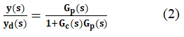
From Eq. (1) and Eq. (2), where y(s) is the output or response, ysp(s) be the set-point input, and yd(s) is load disturbance are the different variables. The dynamics of numerous chemical industrial processes, such as the bioreactor, dimerization reactor, and continuous stirred tank reactor (CSTR), can be linearised as the unstable process of first order transfer functions 12.

where τ is the system’s time constant, θ is the process time delay, and Kp is the plant gain. By defining the intended transfer function for set-point changes, the controller Gc(s) is derived in the form of a Proportional-Integral (PI) controller with first order lead-lag filter in the following section. The aforementioned controller’s transfer function is,

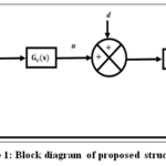 |
Figure 1: Block diagram of proposed structure5 Click here to View Figure |
Proportional-Integral (PI) controller with first order lead-lag filter
Using Eq. (1), the controller may be expressed as follows:

The desired transfer function for set point change in this case is (y/ysp)d . It is important to select a transfer function that will allow the controller to be physically realizable and to explicitly acquire the unknowns in terms of the parameters of the plant.
Additionally, applying the direct synthesis approach the expected desired transfer function is,

Where the λ is the parameters to be selected and based on that controller parameters, η is calculated. Based on Equation (3), Gc (s) can be derived as

For simplification Pade’s first order approximation e-θs = 1 – 0.5θs/1 + 0.5θs is considered and corresponding expression for controller is obtained as,

After simplifying the controller expression and rearranging it is obtained as
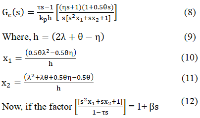
Now, Equating the co-efficient of each term of Eq. (12),

From Eqs. (9), (10), (11) and (13), we obtain
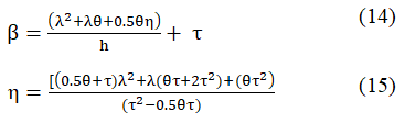
The final controller equation formulated in standard PI structure as given by

Therefore, comparing the Eq. (8) and (16), and considering Eqs. (9), (10), (11), (14) and (15), the PID parameters can be obtained as follows,
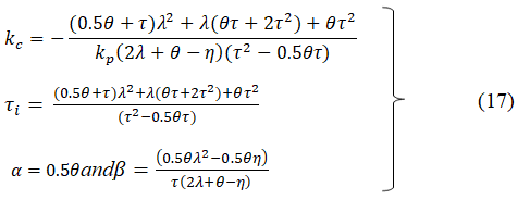
Here, (ηs +1) in the numerator of the Eq. (6) results as overshoot in the output response of set point. To control the unwanted overshoot, a first-order reference filter might be used 23. In this publication, a first-order reference filter of 1/((ηs+1)) can be used to control the same.
Tuning parameters selection
Choosing the tuning parameter (λ) is a crucial and difficult task. In order to attain the intended outcomes and functionality, controller settings are acquired. The computation of (λ) selection for various unstable first order is done after maintaining the intended maximum sensitivity as

The suggested work selects λ such that the maximum sensitivity remains at 2, allowing for justifiable performance or greater values for processes with differing natures. Some factors like load disturbances, noise, and model–plant mismatch are inevitable and must be considered for reliable performance.
Stability and Robustness validation
The stability and robustness validation is performed in the presence of undesired load changes and uncertainties in the process model. If the infinity norm of product of complementary sensitivity function,
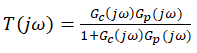
and maximum admissible multiplicative uncertainty, lm (s = jω) is less than unity, the designed structure is robustly stable 24.

In the event where the time delay is unclear, the tuning parameter λ ought to be chosen in a way that,

And the process uncertainty can be represented as,

Here, Gm (jω) represents the model of the unstable process. For UFOPTD processes, if uncertainty exists in the process gain, the tuning parameter, λ should be selected appropriately to ensure robust stability and satisfactory closed-loop performance under gain variations such that,

Likewise, in the presence of uncertainty in τ, an analogous analysis shows that the tuning parameter λ should satisfy the following constraint.

For achieving robust stability and robust performance of the closed-loop system, the constraints specified in (13) and the following condition must be satisfied5.

Here, wm(jω) is bound on the sensitivity function, S(jω) = 1 – T(jω) in the presence of uncertainty. Controller tuning must ensure that the robust stability and robust performance inequalities specified in (19) and (24) are fulfilled.
Simulation study
It is widely acknowledged that the choice of the closed-loop tuning parameter, λ has an intrinsic trade-off. For stable processes, smaller values of λ typically lead to quicker responses and higher performance in rejecting disturbances, whereas larger values promote improved stability and robustness. The conventional guideline is not always applicable to unstable processes, rendering the selection of λ particularly critical in such cases. To provide a systematic procedure for choosing λ, this study adopts the parameter Ms being the maximum sensitivity, is a widely used robust performance measure, analogous to the gain margin (GM) and phase margin (PM). Moreover, it is related to these classical stability margins through the inequalities by GM ≥ Ms/(Ms – 1) and PM ≥ 2sin-1 (1/2Ms). In this study, for the process Gp(s) = e-0.4s/s-1 is considered for selection of tuning parameter based on robustness analysis. The maximum sensitivity function, Ms, is first evaluated as a function of the controller tuning parameter λ as in Eq. (18). This relationship provides a direct guideline for selecting appropriate values of λ that achieve a desired trade-off between robust stability and closed-loop performance. The resulting plot, shown in Fig. 2, reveals that for a given specified value of Ms, two distinct values of λ can exist. The bigger value of λ is usually better since it makes the system more robust against modeling errors and outside influences while avoiding overly aggressive control action. Based on this study, the tuning parameter λ = 0.45 is chosen, which offers a good balance between stability and responsiveness.
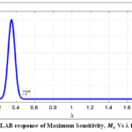 |
Figure 2: MATLAB response of Maximum Sensitivity, Ms Vs λ for Example 123 Click here to View Figure |
Based on the selected parameter, robustness is further validated by examining the variation of Ms with respect to the normalized time-delay ratio θ/τ for different choices of λ, as presented in Fig. 3. This analysis is particularly significant because the ratio θ/τ represents uncertainty in process dynamics and is commonly encountered in real industrial systems. The obtained results demonstrate that for λ = 0.45 and λ = 0.6, the sensitivity function Ms remains nearly constant over a broad range of θ/τ, indicating robust closed-loop stability and consistent performance even under significant variations in process dead time and time constant. In contrast, smaller values of λ lead to larger variations in Ms, suggesting increased sensitivity to parameter uncertainties and reduced robustness margins.
To further verify the robustness characteristics in the frequency domain, the magnitude of the output sensitivity function is analysed for different values of λ, as shown in Fig. 4. This analysis highlights the impact of tuning on noise amplification and high-frequency behavior of the control system. The results indicate that increasing λ beyond 0.45 results in greater attenuation of high-frequency disturbances but at the expense of reduced closed-loop bandwidth and a noticeably slower transient response. Specifically, selecting λ = 0.6 or higher leads to sluggish time-domain performance with longer settling times and decreased responsiveness. Therefore, while larger values of λ improve robustness, they degrade dynamic performance, establishing a clear trade-off. Considering both time-domain response characteristics and robustness margins, the tuning parameter λ = 0.45 is therefore selected as the optimal value for the subsequent controller design and tuning stages.
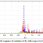 |
Figure 3: MATLAB response of variation of Ms with respect to θ/τ for Example15 Click here to View Figure |
To quantitatively demonstrate the effectiveness of the proposed tuning method, standard performance indices including maximum sensitivity Ms, integral error criteria (IAE, ITAE, and ISE), and total variation (TV) of the control signal are evaluated and compared with existing methods under both nominal and perturbed conditions. The approach is validated through three benchmark examples, where system performance is assessed after controller tuning and robustness verification. The TV index, computed from the discretized control signal as
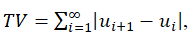
reflects the smoothness of the control action. The results summarized in Table 2 confirm that the proposed method consistently yields lower performance indices, indicating superior tracking accuracy, robustness, and smoother control effort. Additionally, Fig. 4 shows that the robust stability condition is satisfied for λ = 0.45 under a 1 time-delay uncertainty, validating the suitability of the selected tuning parameter.
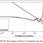 |
Figure 4: MATLAB response of T(jω) Vs frequency for Example 125 Click here to View Figure |
Example 1: A first-order unstable process with a transfer function of Gp(s) = e-0.4s/s-1 is examined. The proposed method is tuned at λ = 0.45 in order to keep Ms = 3, the suggested PI controller parameters of proposed methods are obtained as, Kc = 2.5414, Ti = 2.1104, α = 0.2 and β = 0.0466. Shamsuzzoha & Lee, 2008 26 controller parameters are Kc = 0.4615, Ti = 0.2667, Td = 0.1, a = 1.5779 and b = 0.1053. According to Vanavil et al., 2015 10,


with set point filter of 1/(0.1251s+1) for the aforementioned process model has been published by Ravi Kishore & Padma Sree, 2018 4. At t = 10, a load disturbance of 0.5 and a set point input of unit magnitude are applied.
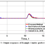 |
Figure 5: Output responses of Example 1 under perfect model Click here to View Figure |
Comparing and demonstrating the closed loop performance, the aforementioned outcomes are superior to or equivalent with alternative techniques. Figs. 5 and 7 explains the closed loop performance under nominal condition, while Table 2 provides the performance metrics in terms of ISE, IAE, ITAE, and TV values. Control signal of the proposed method is explained in Fig. 6. It is clear from Figs. 5 to 7 and Table 2, that the proposed method performs better than the control algorithm proposed in 4, 10because they produce reduced TV, ITAE, ISE, and IAE values, produces a smoother and efficient response.
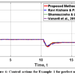 |
Figure 6: Control actions for Example 1 for perfect model Click here to View Figure |
Table 1: Design analysis of various control methods
| Control methods | Design structure | Points to be noted |
| Proposed PI controller | PI with first order filter of lead-lag | Uses one tuning parameter to obtain Four unknown |
| Kishore and Sree4 | PID with filter of first order lead-lag | MDPP techniques used to find five unknown parameters |
| Zhang et al., 2020 16 | PID with first order lead-lag | Three unknown parameters and one tuning/design parameter |
| Chakraborty et al., 201719 | An I-PD controller structure is used | Three unknown parameters in two design steps with one tuning/design parameter |
| Peker & Kaya, 2023320 | An I-PD with set-point filter | Four unknown parameters with one tuning parameter |
Table 2: Performance indices of Example 1.
| Method Name | Nominal | +10% in θ | ||||||||
| ISE | IAE | TV | ISE | IAE | TV | |||||
| Proposed | 0.28 | 1.4 | 8.3 | 4.6 | 0.28 | 1.42 | 8.6 | 6.4 | ||
| Kishore and Sree 4 | 1.4 | 2.2 | 7.4 | 17 | 1.6 | 2.2 | 7.4 | 18.9 | ||
| Shamsuzzoha & Lee, 200826 | 0.2 | 1.1 | 5.4 | 5.1 | 0.22 | 1.1 | 5.5 | 5.9 | ||
| Vanavil et al., 201510 | 0.26 | 1.44 | 8.2 | 4.21 | 0.25 | 1.4 | 8.1 | 4.5 | ||
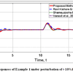 |
Figure 7: responses of Example 1 under perturbation of + 10% Kp, and T. Click here to View Figure |
Fig. 7 illustrates the process parameters affected by responses under such conditions. To assess system resilience, plats apply perturbations of +10%, T and Kp. The proposed controller meets both the robust performance and robust stability requirements with the recommended value of λ.
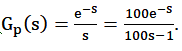
Example 2: An integrating process is considered to verify the proposed method discussed in 16, 19, 20 after simple mathematical modification, .
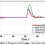 |
Figure 8: Responses for Example 2 for perfect model. Click here to View Figure |
Chakraborty et al., 2017[24] designed an I-PD controller with parameters as Kp = 0.844, Ti = 3.55 and Td = 0.482. Peker & Kaya, 2023 [25] suggested PID controller with its controller parameters as Kp= 0.6340, Ti = 4.4147, Td = 0.1533, and f = 0.3814. A PID of Kp = 0.8916, Ti = 4.3673 and Td = 0.4267 was suggested by Zhang et al., 2020 [17] to regulate the integrating process. The same value of maximum sensitivity Ms = 2 used in all other approaches was used to compare the outcomes of the proposed strategy.
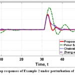 |
Figure 9: Closed loop responses of Example 2 under perturbation of +10% in Kp and θ. Click here to View Figure |
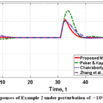 |
Figure 10: Responses of Example 2 under perturbation of -10% in Kp and θ. Click here to View Figure |
Applying the similar approach for tuning purpose and observe that for λ = 1.3, it gives the most suitable value. The controller parameters are obtained as, Kc = 4.2668, Ti = 4.7020, α = 0.5 and β = 0.1534. The suggested technique is being simulated after a set point input of one unit step is applied, and the proposed method’s output response is tested using a load disturbance of positive magnitude of 0.5.
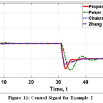 |
Figure 11: Control Signal for Example 2 Click here to View Figure |
Figure 8 displays the closed loop response of the approaches, and Table 3 reports the associated performance metrics. Set point filters are used to compensate for unwanted overshoot in the response.
Table 3: Performance values for Example 2
| Method Name | Nominal | +10% in Kp and θ | -10% in and θ | |||||||||||
| ISE | IAE | ITAE | TV | ISE | IAE | ITAE | TV | ISE | IAE | ITAE | TV | |||
| Proposed | 0.92 | 2.9 | 64 | 2 | 1.1 | 3 | 68 | 3.1 | 0.84 | 3 | 65 | 1.7 | ||
| Peker & Kaya, 202320 | 5.5 | 8.2 | 144 | 2.2 | 6 | 9.4 | 195 | 3.2 | 5.3 | 7.8 | 132 | 1.8 | ||
| Chakraborty et al., 201719 | 3.7 | 5.9 | 84 | 1.6 | 3.7 | 5.7 | 80 | 3.2 | 3.7 | 6.2 | 89 | 1.4 | ||
| Zhang et al., 202016 | 2.6 | 5.5 | 93.2 | 2.7 | 2.9 | 5.5 | 93 | 1.87 | 2.4 | 5.4 | 94 | 2.1 | ||
The approach given in Table 3 has TV values that are either minimal or comparable to other ways. Figs. 9 and 10 show the plots of the justified perturbation, which is within ±10% of the Kp and θ is easily controlled by the controller design. control signals shown in Fig. 11 suggested that method yields smooth control signal. Satisfactory value of robustness is attained by the suggested controller. Indices like ISE, IAE, and ITAE are obtained with the aforementioned uncertainties present. The primary advantage of the suggested strategy is that good tuning leads to improved overall performance even with simpler control.
Application to Nonlinear System
The differential Eq. (25) deals with the non-linear dynamics of isothermal chemical reactor as shown in Fig. 127, 27

Here Q, and CF indicate the inlet flow rate and inlet concentration, C respectively, while represents the reactor outlet concentration. The model parameters are Q = 0.0333 L/s, k1 = 10 L/s, k2 = 10 L/mol, and reactor volume V = 1L . The desired steady state is C = 1.316, corresponding to a nominal feed concentration of CF = 3.288 mol/L. first the non-linear process is linearised, and the feed concentration is taken as the controlled variable. Considering a process time delay of 20sec, the approximated model is obtained as,

This linear model is used for controller design, but the resulting controller is tested on the original nonlinear model (20). By setting λ = 1.75θ in Eq. (17), controller settings are obtained as Kc = 1.1204, τi = 121.62 τd = 0, α = 10 and β = 3.7577. Raja and Ali 8 uses PI plus PD structure with

Onat, Cem 9 suggested a PI-PD structure with inner loop as a PD type (111.26)s + 666/s+100 & outer loop with PI type (0.4289)s + 0158/s.
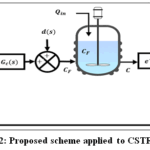 |
Figure 12: Proposed scheme applied to CSTR process2 Click here to View Figure |
To evaluate the effectiveness, a unit-step change in the set point is introduced, and a unit disturbance is applied at t = 1000s. The corresponding closed-loop responses of the outlet concentration are depicted in Figs. 15 and 16. These figures provide a comparative assessment of the proposed PI controller with the methods reported in 8 and 9. Figure 13 illustrates the set-point tracking performance. As seen from the plot, the approach in 8 and 9 demonstrates a delayed dynamic response. The output takes a considerably long time to rise and settle near the desired value, indicating poor responsiveness. The method proposed by 8 shows an improved rise time and achieves the set point more quickly. However, this faster response is obtained at the cost of excessive control effort, which is evident from the significantly high total variation (TV) listed in Table IV. High TV indicates aggressive control actions that may cause actuator wear, increased energy consumption, and potential instability in real-time operation.
Table 4: Performance values of Example 3
|
Method Name |
Nominal | in | ||||||
| ISE | IAE | TV | ISE | IAE |
TV |
|||
|
Proposed |
2168 | 728 | 202100 | 18.5 | 2251 | 729 | 200700 |
20.2 |
|
Raja and Ali 8 |
3127 | 801 | 107000 | 32 | 3255 | 812 | 109000 | 46.2 |
| Onat, Cem 9 | 4491 | 1130 | 209500 | 18.5 | 4582 | 1133 | 209200 |
21.9 |
Also, the response obtained using the proposed PI controller approach gives a balanced and comparable result. The output reaches the desired value in a reasonable time without excessive control effort as seen in Fig. 14 and even settles easily after the disturbance, and is notably shorter than that of the method in 9.
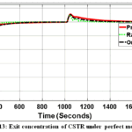 |
Figure 13: Exit concentration of CSTR under perfect modelling. Click here to View Figure |
To further verify robustness, a model mismatch of +20% in the process delay θ is introduced, and the resulting system behaviour is presented in Fig. 15.
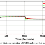 |
Figure 14: Inlet concentration of CSTR under perfect modelling. Click here to View Figure |
From Fig.15, it is evident that the proposed controller maintains stable operation even in the presence of significant parameter uncertainty. Also, the proposed method is verified with the application of noise having variance of 1 and sample time 0.1, as shown in Fig. 16. From Figs. 13-16, proposed method results balanced speed and robustness highlights the improved disturbance-handling characteristics of the proposed scheme. The transient behaviour remains well-behaved, and the steady-state value is achieved with only a marginal deviation. This confirms that the proposed control design provides adequate tolerance against modelling errors, which is essential for real-world chemical processes where exact parameters are seldom known.
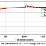 |
Figure 15: Exit concentration for for CSTR system Click here to View Figure |
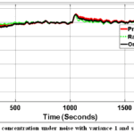 |
Figure 16: Exit concentration under noise with variance 1 and sample time 0.1 Click here to View Figure |
Conclusion
Industrial processes with an unstable nature use a proportional integral (PI) controller with a lead-lag filter. The direct synthesis method is used to get controller parameters, which are then changed to fit the desired maximum sensitivity range. It is proposed and tested that the right design parameter values will cause a justified change in the plant parameters. Using the proposed control design method, controller parameters are first obtained for the linearised model of non-linear CSTR, and then validated on the corresponding non-linear CSTR by making simple changes to the function. Performance improvement in all the three examples approved the efficacy of suggested technique. The proposed PI controller, which have only four unknowns, worked better or comparable as well as some newer methods. Proposed single loop control is better than recently reported controllers and is easier to implement with the right tuning.
Acknowledgement
Authors would like to thank NCE Chandi, DCE Darbhanga, GEC Nawada and GCE Gaya for providing opportunity to do research work.
Funding Sources
The author(s) received no financial support for the research, authorship, and/or publication of this article.
Conflict of Interest
The author declares that there are no known competing financial interests or personal relationships that could have appeared to influence the work reported in this paper.
Data Availability Statement
Data sharing is not applicable to this article. No any datasets are analysed or generated during the current study
Ethics Statement
This research did not involve human participants, animal subjects, or any material that requires ethical approval
Authors/Co-author names and affiliations and their Contributions:
- Sanjay Kumar: Contributions- Conceptualization, simulations, theoretical development, result analysis, manuscript writing, Validation
- Ishwar Chandra Thakur: Darbhanga College of Engineering, Darbhanga: Contributions-Theoretical development, result analysis
- Mr. Akash: Government Engineering College, Nawada: Contributions-Conceptualization,result analysis, manuscript writing
- Prabhat Kumar: Darbhanga College of Engineering, Darbhanga: Contributions- Theoretical development, result analysis, manuscript writing
- Md. Akram Alam: Gaya College Engineering College, Gaya: Contributions – Theoretical development, result analysis, manuscript writing
References
- Kumar S and Ajmeri M. Double loop fractional order IMC for integrating plants with inverse characteristics and delay. In: 2023 IEEE 3rd International Conference on Smart Technologies for Power, Energy and Control (STPEC) 2023, pp.1-6. IEEE.
CrossRef - Kumar S, Ajmeri M and Mehta U. Dual-loop fractional-order IMC structure for unstable systems to handle ramp input signals. IEEE Access 2025.
CrossRef - Kumar M, Prasad D and Singh RS. Performance enhancement of IMC-PID controller design for stable and unstable second-order time delay processes. Journal of Central South University 2020; 27: 88-100.
CrossRef - Ravi Kishore C and Padma Sree R. Design of PID controllers for unstable systems using multiple dominant poleplacement method. Indian Chemical Engineer 2018; 60: 356-370.
CrossRef - Vanavil B, Chaitanya KK and Rao AS. Improved PID controller design for unstable time delay processes based on direct synthesis method and maximum sensitivity. International Journal of Systems Science 2015; 46: 1349-1366.
- Vijayan V and Panda RC. Design of PID controllers in double feedback loops for SISO systems with set-point filters. ISA transactions 2012; 51: 514-521.
CrossRef - Ajmeri M and Ali A. Two degree of freedom control scheme for unstable processes with small time delay. ISA transactions 2015; 56: 308-326.
CrossRef - Lloyds Raja G and Ali A. New PI-PD Controller Design Strategy for Industrial Unstable and Integrating Processes with Dead Time and Inverse Response. Journal of Control, Automation and Electrical Systems 2021; 32: 266-280. DOI: 10.1007/s40313-020-00679-5.
CrossRef - Onat C. A new design method for PI–PD control of unstable processes with dead time. ISA transactions 2019; 84: 69-81.
CrossRef - Vanavil B, Anusha AVNL, Perumalsamy M, et al. ENHANCED IMC-PID CONTROLLER DESIGN WITH LEAD-LAG FILTER FOR UNSTABLE AND INTEGRATING PROCESSES WITH TIME DELAY. Chemical Engineering Communications 2014; 201: 1468-1496. DOI: 10.1080/00986445.2013.818983.
CrossRef - Karan S and Dey C. Simplified tuning of IMC based modified smith predictor for UFOPDT processes. Chemical Product and Process Modeling 2021; 16: 21-40.
CrossRef - Chanti Babu D, Santosh Kumar DB and Padma Sree R. Tuning of PID Controllers for Unstable Systems Using Direct Synthesis Method. Indian Chemical Engineer 2017; 59: 215-241. DOI: 10.1080/00194506.2016.1255570.
CrossRef - Kumar S and Ajmeri M. Enhanced design of PI controller with lead-lag filter for unstable and integrating plus time delay processes. Chemical Product and Process Modeling 2023; 18: 793-809.
CrossRef - Rahul BS and Ajmeri M. Enhanced design of PID controller and noise filter for second order stable and unstable processes with time delay. Chemical Product and Process Modeling 2022.
CrossRef - Begum KG, Rao AS and Radhakrishnan T. Enhanced IMC based PID controller design for non-minimum phase (NMP) integrating processes with time delays. ISA transactions 2017; 68: 223-234.
CrossRef - Zhang W, Cui Y and Ding X. An improved analytical tuning rule of a robust PID controller for integrating systems with time delay based on the multiple dominant pole-placement method. Symmetry 2020; 12: 1449.
CrossRef - Lloyds Raja G and Ali A. New PI-PD controller design strategy for industrial unstable and integrating processes with dead time and inverse response. Journal of Control, Automation and Electrical Systems 2021; 32: 266-280.
CrossRef - Kaya I. Integral-proportional derivative tuning for optimal closed loop responses to control integrating processes with inverse response. Transactions of the Institute of Measurement and Control 2020; 42: 3123-3134.
CrossRef - Chakraborty S, Ghosh S and Kumar Naskar A. I–PD controller for integrating plus time‐delay processes. IET Control Theory & Applications 2017; 11: 3137-3145.
CrossRef - Peker F and Kaya I. Maximum sensitivity (Ms)-based I-PD controller design for the control of integrating processes with time delay. International Journal of Systems Science 2023; 54: 313-332.
CrossRef - Panda RC. Synthesis of PID controller for unstable and integrating processes. Chemical Engineering Science 2009; 64: 2807-2816.
CrossRef - Kaya I and Cengiz H. Optimal tuning of PI/PID controllers for integrating processes with inverse response. In: 2017 21st International Conference on System Theory, Control and Computing (ICSTCC) 2017, pp.717-722. IEEE.
CrossRef - Kumar S and Ajmeri M. Analytically designed dual-loop fractional-order IMC for integrating plants with inverse behavior. International Journal of Dynamics and Control 2024: 1-15.
CrossRef - Ajmeri M and Ali A. Analytical design of modified Smith predictor for unstable second-order processes with time delay. International Journal of Systems Science 2017; 48: 1671-1681.
CrossRef - Ranjan A and Mehta U. Fractional-order tilt integral derivative controller design using IMC scheme for unstable time-delay processes. Journal of Control, Automation and Electrical Systems 2023; 34: 907-925.
CrossRef - Shamsuzzoha M and Lee M. Analytical design of enhanced PID filter controller for integrating and first order unstable processes with time delay. Chemical Engineering Science 2008; 63: 2717-2731.
CrossRef - Begum KG, Rao AS and Radhakrishnan TK. Novel IMC filter design-based PID controller design for systems with one right half plane pole and dead-time. International Journal of Automation and Control 2020; 14: 423-444.
CrossRef
 PlumX:
  Views: 394 Views
  PDF Downloads: 138
 Accepted on: 06 Mar 2026
Second Review by: Dr. Asif Khan
Final Approval by: Dr. Tanay Pramanik


ISSN Online: 2231-5039