Waters Metallic Typology of Oued Tisslit-Talssint (Morocco Oriental)
H. Taouil1, H. Hanafi2, S. Elanza3, S. Ibn Ahmed1, M. Aboulouafa1*and H. Lemacha4
1Laboratoire des Matériaux, d’Electrochimie et d’Environnement. Université Ibn Tofail. Département de Chimie, B.P. 133, 14000 Kenitra, Maroc.
2Laboratoire de Physico-chimie des Matériaux et Environnement. Université Abdelmalek Essaâdi, Faculté des Sciences, B.P. 2121, Tétouan, Maroc.
3Laboratoire de Synthèse Organique et Procédés d`Extraction, Université Ibn Tofail. Département de Chimie, B.P. 133, 14000 Kenitra, Maroc.
4Laboratoire de Géologie Appliquée, Géomantique et Environnement. Département de géologie. Faculté des Sciences Ben M’sik, Université Hassan II de Casablanca, Maroc.
Corresponding Author. E-mail: Mohammed.aboulouafa@uit.ac.ma
DOI : http://dx.doi.org/10.13005/ojc/330324
In The purpose of the management and conservation of the aquatic environment of WadiTislit-Talssint, a principal components analysis of eight heavy metals, has been conduct during the period of low water (May 2011). The visualization of results has allowed us to show that, Mn, Fe and Ni are positively correlated to the axis F1, unlike the heavy metals: Co, Cu, Cd and Zn which is associated with this axis negatively. On the main axis F2, only the problem that a positive correlation, as well the application of the principal component analysis on these results, shows that we have two groups of stations: a first group of stations in the positive part of the F axis1, characterized by waters with high concentrations (Mn, Fe and Ni), in the stations S0 and sc1.A second group of stations in the negative part of the F axis1, characterized by waters with high concentrations (Cu, Cd, Zn, and CO in the stations (SR1 and SR2). This enrichment in metallic elements is to put in relationship with the inputs of wastewater and solid waste of the commune of Talssint, flowing upstream of the stations SR1 and directly at the level of the station SR2.
KEYWORDS:ACP; metal typology; OuedTisslit-Talssint
Download this article as:| Copy the following to cite this article: Taouil H, Hanafi H, Elanza S, Ahmed S. I, Aboulouafa M, Lemacha H. Waters Metallic Typology of Oued Tisslit-Talssint (Morocco Oriental). Orient J Chem 2017;33(3). |
| Copy the following to cite this URL: Taouil H, Hanafi H, Elanza S, Ahmed S. I, Aboulouafa M, Lemacha H. Waters Metallic Typology of Oued Tisslit-Talssint (Morocco Oriental). Orient J Chem 2017;33(3). Available from: http://www.orientjchem.org/?p=33535 |
Introduction
The quality of surface waters is influenced by natural processes (erosion, precipitation, evaporation) and by human activity (agriculture, urban and industrial waste water). [1] Thus the pollution of freshwater in Morocco is undoubtedly one of the most disturbing aspects of environmental degradation. Indeed, the water reserves are subject to significant operational, which we run the greatest dangers in exposing Morocco to adverse consequences. Among the chemical substances likely to be at the origin of the deterioration of the quality of the waters, are the heavy metals [2]. Some have a high toxicity. They differ from other chemical pollutants, by their low biodegradability and their important power of bioaccumulation along the trophic chain; this can cause significant environmental damage. Since the previous work has shown that the anthropogenic activity remains the primary cause of the degradation of the quality of natural waters [3]. We must, therefore, be very aware of the importance of the risks that this pollution poses in the areas sub-Saharan, Saharan and of the region of the Eastern Morocco” Talssint”. Indeed, we have counted a large number of wastewater discharges, direct in Wadi Tislit-Talssint. Total releases is discharged directly onto the river without any prior pre-treatment, a complete diagnosis of the current situation of the metal pollution and stringent monitoring, which are proving to be a great need in order to be able to judge the quality of these waters and its impact on the environment. It is in this perspective that we have proceeded to the study of the impact of the waters of the studied environments on the state of the environment of the commune of Talssint [4-7]. In this context we have to make a principal components analysis of heavy metals of the waters of Oued Tislit-Talssint was made based on samples were taken during the course of two companions during a period of low water (month of May and June 2011). In this context, the use of different multivariate statistical techniques (principal components analysis, classification methods) for data interpretation seems an interesting solution for a better understanding of water quality and ecological status of environments studied. The choice of Principal Component Analysis Module System Software for Data Analysis (SFDA), allowed us to visualize the following results:
The correlation matrix of variables;
The table of the correlation matrix own values and the explanation percentage of each own value;
A plane of the variables projection.
Therefore, the work will reside in the interpretation of the different results.
Expérimental
Study area
The region of Talssint belongs to the domain of the High Atlas Moroccan Oriental, part of the eastern region, putting the contact this last and the regions of Tafilalt-Meknes and Fes-Boulmane. As well the region of Talssint can be divided into two units: to the west to settle the mountains of the High Atlas Oriental, with altitudes that exceed 2000 m, including the highest are: Jbel Falchou (2303m), Jbel Skendis (2173m), and Jbel Mechkakour (212.2 m). In the center and to the east of the country, the area of the high plateaux which covers two thirds of the region of the oriental with altitudes between 1000 and 1650 m. Talssint administratively belongs to the province of Figuig, in the south of the region of the oriental. Its surface covers 11,000 km2, limited to the north by Missour and Ouatat-al Haj, by Benitadjit to the South, Maatarka to the east and by Gourrama to the west.
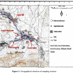 |
Figure 1: Geographical situation of sampling . Click here to View table |
Bioclimatic Plan
On the bioclimatic plan, the region is characterized by pre-Saharan and Saharan environments. Temperatures are high in summer and very cold in winter, the mean minimum of the coldest month (January) is – 5 °C and the average maximum temperature of the warmest month (July) is 47 °C. Annual rainfall average was around 245 mm for the 1983/2007 period with significant inter annual variations, it is about 500 mm for the period 2008/2010: recorded extremes are 61 mm in 1998/99 and 684 5 mm in 2009/2010 [8].
Data processing Methods
In order to achieve a comprehensive synthesis of various results and develop a spatial structure to identify phenomena determinants the functioning of aquatic system, we proceeded to a Multidimensional Analysis which is part of the descriptive statistics. We have submitted all of the data, collected to a principal components analysis (ACP) which allows analyzing data tables of quantitative Digital to reduce the dimensionality in finding a new set of variables smaller than the whole of the variables, which nevertheless contains most of the information. The principal components are obtained by diagonalization of the matrix of two different correlations. This diagonalization defines a set of own values whose observation for each component allow to determine the number of graphics to be examined [9]. The final phase of the CPA is a graphical representation that allows previewing the results that digital expressions do not provide. . In effect the ACP has for objective to present, in a graphic form the maximum of the information contained in a data table, based on the principle of double projection on the factorial axes [10]. As well the ACP allows explaining the structure of the correlations or covariances using linear combinations of the original data. As well its use allows to reduce and to interpret the data on a reduced space [11]. The correlations between variables and axes and projection of variables in F1 and F2 axes of space were obtained with STATISTICA Software 10. In effect the data analyzes of heavy metals are processed by this software, as well the choice of this software is justified by its simplified mode of use, its interface enriched by Excel for data entry.
Results and discussion
Correlation matrix between variables
In our example, some variables are correlated positively and others are negatively correlated. So heavy metals that are positively correlated move in the same direction; that is, the increase of one affects the increase of the other, then the variables that are negatively correlated vary in opposite directions; that is to say the increase in one leads to the decrease in the other.
Table 2: The correlation matrix between the variables studied during this study.
| Variables | Pb | Cd | Cu | Ni | Zn | Mn | Co | Fe |
| Pb | 1 | |||||||
| Cd | 0.633 | 1 | ||||||
| Cu | 0.589 | 0.984 | 1 | |||||
| Ni | 0.056 | -0.542 | -0.606 | 1 | ||||
| Zn | 0.836 | 0.840 | 0.824 | -0.478 | 1 | |||
| Mn | 0.051 | -0.516 | -0.596 | 0.975 | -0.487 | 1 | ||
| Co | -0.123 | 0.398 | 0.401 | -0.285 | -0,037 | -0.134 | 1 | |
| Fe | 0.375 | -0.337 | -0.439 | 0.885 | -0.117 | 0.871 | -0.475 | 1 |
Positive correlation
The positive correlations (variation of the metals concentrations in the same direction) and after the strong Degrees of correlation between the variables studied, can classify them into four groups as suite (Table 3).
Table 3: Ranking of the positive correlation of some heavy metals studied during the present study.
| correlation degree | 0.975 à 0.984 | 0.824 à 0.885 | 0.375 à 0.398 | 0.051 à 0.056 |
| Variables | Mn/NiCu/Cd | Zn /CuZn/ PbZn/ CdFe /MnFe/ Ni | Fe/ PbCo /Cd | Ni /PbMn/ Pb |
Negative correlation
The negative correlations which vary in two opposite directions where one of the variables increasing led to the decrease of the other and after the low correlations between the groups of variables studied, we can classify them as follows (Table 4):
Table 4: Ranking of the negative correlation of some heavy metals studied during the present study.
| Correlation degree | -0.596 à -0.516 | -0.487 à 0.439 | -0.134 à – 0.117 |
| Variables | Ni/ CdMn/ CdMn/Cu | Fe/ CuZn/ NiMn /ZnFe /Co | Co/PbFe/ ZnCo/Mn |
Diagonalization of the correlation matrix
Table 5 and Figure 2 provide the diagonalization of the correlation matrix. The second line indicates the specific values of the correlation matrix. The third line tells us the percentage explained by each own value.
Table 5: Diagonalization of the correlation matrix of the studied variables.
| F1 | F2 | F3 | F4 | F5 | F6 | |
|
Own value |
4.604 | 2.799 | 1.211 | 0.324 | 0.049 | 0.012 |
| Variability (%) | 51.161 | 31.095 | 13.459 | 3.600 | 0.548 | 0.137 |
| % cumulated | 51.161 | 82.256 | 95.714 | 99.314 | 99.863 | 100.000 |
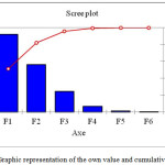 |
Figure 2: Graphic representation of the own value and cumulative variability. |
Representation of Variables and Variable Circle
The coordinates of the variables in the axial planes F1, F2, …, F6 shown in Table 6 show the representation of variables in the (factor 1, factor 2) explaining 82.26% of the initial inertia. To each variable is assigned a point on a coordinate factor axis is a measure of the correlation between this variable and the factor (F1 Axis or F2 Axis). ) Example the coordinated on the Axis 1 of the variable lead concentration is -0.13 and the one on the Axis 2 is 0.561 (Table 6). By projection on a factorial design, the variables are part of a circle of radius 1. Therefore to facilitate the visualization of the clouds of points, it was projected in a space to 2 dimensions. The percentage of inertia explained by the two axes forming a plan (F1 and F2) is 82.26% of the total variance (Figure 2). These two axes are taken into consideration for the description of the distribution of the variables on the main plan. The first and the second axis explained, respectively 51.16% and 31.10% of the total inertia.
Table 6: correlations between variables and factors.
| F1 | F2 | F3 | F4 | F5 | F6 | |
| Pb | -0.130 | 0.561 | -0.141 | -0.063 | -0.501 | -0.474 |
| Cd | -0.392 | 0.281 | 0.129 | 0.360 | 0.427 | 0.316 |
| Cu | -0.415 | 0.230 | 0.106 | 0.361 | -0.208 | 0.006 |
| Ni | 0.419 | 0.204 | 0.071 | 0.426 | -0.389 | 0.551 |
| Zn | -0.333 | 0.380 | -0.237 | -0.220 | 0.128 | 0.201 |
| Mn | 0.415 | 0.216 | 0.215 | 0.257 | 0.019 | -0.245 |
| Co | -0.170 | -0.052 | 0.842 | 0.013 | 0.026 | -0.245 |
| Fe | 0.351 | 0.367 | -0.147 | 0.182 | 0.594 | -0.315 |
The previous work has shown that the angle between variables is less than 90 °; this suggests that these variables are positively correlated with each other while between the angle is greater than 90 °; this suggests that these variables are negatively correlated with each other. From Figure 3 the Mn, Fe and Ni are positively correlated to the axis F1, unlike heavy metals: Co, Cu, Cd and Zn which is associated with this axis negatively. F2 on the main road, only Pb has a positive correlation.
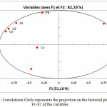 |
Figure 3: Correlations Circle represents the projection on the factorial plane F1-F2 of the variables. |
Table 7: Observations Coordinates of the seven stations
| Observation | F1 | F2 | F3 | F4 | F5 | F6 |
| 1 | 4.488 | 1.842 | -0.299 | 0.252 | 0.084 | 0.001 |
| 2 | 0.312 | -0.579 | 2.402 | -0.563 | 0.063 | 0.023 |
| 3 | -1.610 | 1.783 | -0.548 | -0.356 | -0.276 | 0.162 |
| 4 | -2.979 | 1.966 | -0.005 | 0.263 | 0.241 | -0.127 |
| 5 | 0.449 | -1.566 | -1.337 | -0.890 | -0.023 | -0.119 |
| 6 | -0.106 | -1.261 | 0.399 | 0.825 | -0.357 | -0.087 |
| 7 | -0.553 | -2.186 | -0.611 | 0.469 | 0.269 | 0.148 |
The projection of variables on the I-II plan shows two poles (Figure 3):
– The factor I represents 51.16% of the variance, it is determined by Fe, Mn, Ni, Cu, Cd and Zn.
– Factor II represents 31.10% of the variance and is determined by Pb.
Finally the correlation circle allows seeing, among the old variables, highly correlated variables groups together. So his study is simpler and more informative than the direct analysis of the correlation matrix.
Representation of stations Individuals study
The arrangement of the stations of the Wadi-TislitTalssint in the plane defined by the first and second axis (Figure 4) showed that:
– A first group of stations in the positive part of the F1 axis, characterized by high water concentrations (Mn, Fe and Ni), at stations S0 and SC1.
– A second group of stations in the negative part of the F1 axis, characterized by water with high concentrations (Cu, Cd, Zn and Co) at stations (SR1 and SR2).
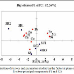 |
Figure 4: Projection of stations and parameters studied on the factorial plane defined by the first two principal components F1 and F2). |
Conclusions
Respect for the environment is a major concern in our societies. Our results will help us to ensure the water quality of Tisli-Talssint River and needs of species occupying this environment. In conclusion, the correlation circle allows seeing, among the old variables, highly correlated variables groups together. So its study is simpler and more informative than the direct analysis of the correlation matrix. Thus, we note that the projection of the variables on the I-II plan shows two poles:
– Factor I represents 51.16% of the variance, it is determined by Fe, Mn, Ni, Cu, Cd and Zn
– Factor II represents 31.10% of the variance and is determined by the Pb As, Mn, Fe and Ni are positively correlated to the axis F1, unlike heavy metals: Co, Cu, Cd and Zn which is associated with this axis negatively. F2 on the main road, only Pb that a positive correlation. Thus the CP has allowed us to highlight similarities or oppositions between the stations and heavy metals. In effect, the application of the principal component analysis on these results shows that we have two groups of stations:
– A first group of stations in the positive part of the F axis1, characterized by waters with high concentrations (Mn, Fe and Ni), at the level of the stations S0 and SC1.
– A second group of stations in the negative part of the F axis1, characterized by waters with high concentrations (Cu, Cd, Zn, and CO) at the level of the stations (SR1 and SR2).
References
- Strobl R.O., Robillard P. D.; “Network design for water quality monitoring of surface freshwaters”: A review. Journal of Environmental Management 2008, 87. 639-648.
CrossRef - Taouil H., Ibn Ahmed S., El Assyry A., Hajjaji N., Srhiri A.; J. Mater. Environ. Sci ,2013. ., 4(4) 502-509.
- Bouras S., Maatoug M., Hellalet B., Ayad N. ; « Quantification de la pollution des sols par le plomb et le Zinc émis par le trafic routier cas de la ville de Sidi Bel Abbes, Algérie occidentale. 2010.,5(20) ,. 11-17.
- Ould Med Fadel K., Taouil H., El Assyry A., Ibn Ahmed. S., Houmani1 H. ; J. Mater. Environ. Sci., 2016.7 (2)
- Taouil H., Ibn Ahmed S., Hajjaji N., Srhir A. ; Sciencelib Editions Mersenne, 2012. 4( 1)2011
- Taouil H., Ibn Ahmed S., ElAssyry A., Hajjaji N., Srhiri A., Elomari F., Daagare A. ; « Int. J. Agric. Policy. Res », 2013. 1(5) 150-155.
- Taouil H., Ibn Ahmed S., E. Rifi1, A. El Assyry. ;” J. Mater. Environ. Sci. 2014.5 (4) 1069-1074.
- Taouil H ; ‘’Les Métaux Lourds dans Le bassin versant du Guir sources de pollution et impact sur la qualité des eaux de surface et souterraines: Cas de Talassent, région du Maroc oriental’’. Thèse, Doctorat, Uni. Ibn Tofail, Faculté des Sciences Kenitra, 2013.
- Lagarde J. ; « Initiation à l’analyse des données, Ed. Duodi. Paris » , 1995, 157
- Maliki. AM. ; « Etude hydrologique hydrochimique et isotopique de la nappe profonde de Sfax (Tunisie). Thèse de Doctorat Fac. Sci. Sfa »x, 2000. 301.
- Taouil H., Ibn Ahmed S., El Assyry A., Hajjaji N., Srhiri A. ; « J. Mater. Environ.,Sci. 2014. 5(1) 177–182.

This work is licensed under a Creative Commons Attribution 4.0 International License.
![]()
A New Edition of Web of Science
Journal Impact Factor
2022: 0.5
Five Year: 0.8
Journal is Indexed in

Cabells Whitelist
![]()