Prediction of vapour-liquid equilibrium for n-alkane fluids

Introduction

An equation of state (EoS) is an analytical expression relating pressure to the volume and temperature. The expression of an equation of state is used [1-3]to describe the volumetric behavior, the vapor-liquid equilibria (VLE), and the thermal properties of pure substances and mixtures. Numerous EoS have been proposed to represent the phase behavior of pure substances and mixtures in the gas and liquid states since van der Waals introduced his expression in 1873.The van der Waals equation provides a qualitatively correct description of the critical point and vapor–liquid equilibrium envelope but for practical applications it is too crude. Nonetheless, it formed a certain basis for developing dozens of empirical equations of state (EoS) used in engineering applications [4-6].

The attraction parameter ‘a’ of van der Waals needed to be made a function of temperature before any cubic EoS was able to do a better job of quantitatively matching experimental data. This was a realization that van der Waals himself had suggested, but no actual functional dependency had been introduced until the Redlich-Kwong [5]EoS. The Redlich-Kong equation of state improved the accuracy of the van der Waals by proposing a temperature dependence attractive term.Thus, the compressibility factors of most empirical equations of state can be expressed as the sum of a temperature-independent term and a temperature-dependent term. Using this functional dependency of temperature in attractive term, the improvement in results for the vapor-liquid equilibrium properties is found significant when the simple but very precise Carnahan–Starling equation has been used. Since these equations of state are cubic in volume, so that the van der Waals concept is retained.

Molecular simulation reveals that the inaccuracies of attractive and repulsive terms respond to some disadvantages to the use of cubic equations of state, andthese inaccuracies are canceled by one other when the EoS’s are employed for the calculation of fluid properties, specifically for the VLE densities.Researchers has emphasizedconsiderably on modeling long and convex molecules in addition to modeling small and simple molecules.Based on theory of Prigogine [7] and Flory [8], an equation for molecules treated as chains of segments, which is called Perturbed-Hard-Chain–theory(PHCT) was expressed by Beret and Prausnitz [9], Donohue and Prausnitz [10]and Gross and Sadowski [11].Large nonspherical molecules such as heavy hydrocarbons and polymers are theoretically modeled as chain like molecules. A chain of tangent hard spheres is the simplest model of this type of molecule. Relaxation of tangency constraint in the tangent hard sphere chains by allowing adjacent hard spheres along the chain to overlap leads to a more realistic model which is known as fused hard sphere chain. Conversely, in the limit, when the center to center reduced length tends to one, the EoS for a fused hard sphere chain reduce to an equation of state of thermodynamic perturbation theory for a tangent hard sphere chain [12].

We have considered different forms for the repulsive part for equations of state [13] of hard spheres such as vdWEoS or CSvdWEoS [18]and also for the equation of state of hard convex body chains such as Boublik [14-16]vdWEoS.For the attractive part of these EoS’s we considered the exponent term to the temperature to zero to reproduce the usual form of vdW or CSvdW or BoublikvdWEoS’s. In this paper,the chemical potential forBoublikvdWEoShas been derived and used to predict the liquid-vapour equilibrium densities of n-alkane fluids. The predictions corresponding to this group of equations of state are within a degree of quality similar to the widely used Carnahan-Starling equation.

This paper is organized as follows. In section 2, we present the expressions for HS and HCB chain EoSandthe corresponding expressions for chemical potentials. This section also includes a table for the critical parameters for n-alkanes.InSection 3 the results, i.e.the diagram for reduced density vs reduced temperature have been plotted and compared with the available experimental data of n-alkane fluids. Conclusions are presented in section 4.

Equations of state for HS and HCB fluids

This section includes three groups of equations of state. The three groups are made on the basis of extensively used add-on separation method of compressibility factor[17-20]as Z= Z_rep+Z_att .The functional dependency of temperature, as introduced by Redlich and Kwong [5], has a power-law form T^-δ  for the attractive part of the EoS’s. For the expression of repulsive part of the EoS’s has any of the three formsvdW, CS and Boublik.Note that in all calculations we set up a new parameter δ  as the temperature-exponent in the attractive term. Notice that the selection to set up δ= 0 regains the original EoS’s.The critical parameters and the analytic expressions for the chemical potential have been determined for the three groups, which allowed us to obtain the VLE densities. Here, for simplicity in calculation we employed the dimensionless variable y=b/4v in place of the molar volume,  with being the co-volume. Here, y=b/4v known as packing fraction[20-23].

As is well known, the chemical potential,μ, can be analytically obtained through [13]:

 

Where, the function φ has the temperature dependency.

The compressibility factor is expressed as, Z= bp/4yRT, where R is the molar universal gas constant. To obtain an analytical expression for μ from equation (1), one requires an analytic expression for the equation of state.

The van der Waals (vdW- ) groups

The compressibility factor for the vdW -δ set of EoS’s is written as

 

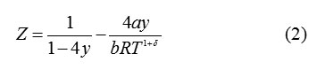
For δ= 0, equn.(2)reproduces the vdWEoS.

Where, λ= 3.375

Using eqns. (1), the expression obtained for chemical potential is:

 

The Carnahan-Starling-van der Waals (CSvdW-δ)group

The CSvdW-δ group assumes its form by replacing the classical vdW repulsive term in eqn.(2) with the CS hard sphereEoS.The functional dependency of temperature for the attractive term of the EoS remains unchanged as in eqn.(2).

The compressibility factor for CS vdW- δ EoS’s can now be written as

 

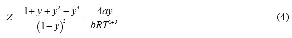
For δ= 0, equn.(4) reproduces the usual form of the CSvdWEoS [17].

Using eqns. (1), the expression obtained for chemical potential is:

 

The Boublik- van der Waals (BoublikvdW- )group

Boublik proposed an equation of state for Hard Convex Bodies [15] as

 

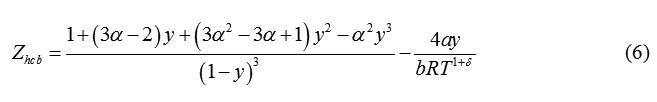
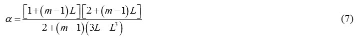
Where, α is the nonsphericity parameter. When, α=1 , eqn. (6) reduces to Carnahan Starling equation. For, other hard convex body, α>1. According to Boublik et al [15], the hard convex body equation can be extended to hard chain molecules of overlapping hard spheres (0.5<L<1) or tangent hard spheres (L=1) with formulation of parameter of nonspherecity as:

 

Using equation(1), the expression obtained for chemical potential is:

 

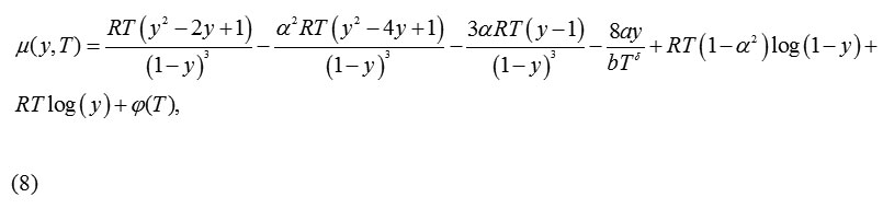
For α= 1, equation (8) reproduces the same equation forthe chemical potentialas that of the CS EoS.

The non-sphericity of the molecule is modeled in terms of the -segments of hard convex bodies. It forms a hard molecule with a chain of freely jointed hard convex bodies. Each n-alkane can be modeledas a chain of m segments of hard HCB.For determination of m-segment value for each n-alkane, one should comprehend that there should be some fundamental phial of our couch of m based on the nature of the HCB. For example, pentane is structured as CH₃CH₂CH₂CH₂CH₃. One may accept that the base unit for pentane is CH₂CH₂ , which could be approximately modeled as ethane (CH₃CH₃₎ Since, two atoms of carbon cannot be approximated as one atom of carbon because of its higher mass as compared to the mass of hydrogen. But for lighter hydrogen one can approximate two hydrogen atoms as one atom or vice versa.Knowing the HCB of ethane and using this base of HCB with m=2.5 to model Pentane. For decane, using the CH₂CH_{2 as}  HCB, m=5. Note that the values guarded bythe base model for the HCB have only sense in modeling the n-alkanes. Using this concept, the value of m has been calculated for each n alkane and is tabulated in Table 1. The table also gives the values of the non-sphericity parameter  as calculated using equation (7).

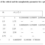Table 1: Values of the critical and the nonsphericity parameter for a given HCB segment m  Click here to View table

 

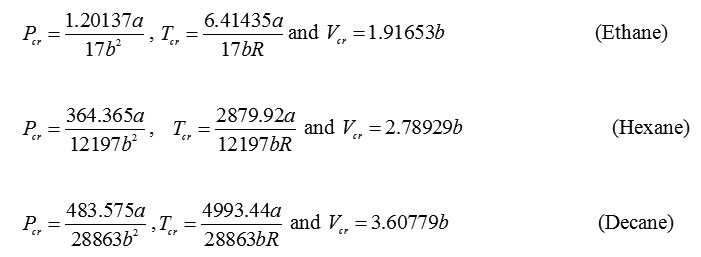
For n-alkanes, when the critical point conditions can be solved to yield the critical parameters. The calculated critical parameters for pressure, temperature and volume for selected n-alkanes are:

Results and discussion

We examined the behavior of the three groups of EoS’s by calculating the VLE densities, and compared them with the experimental data [19] for fluids of n-alkanes.In particular, we calculated the co-existence curvesin the y, versus T, diagram.The calculations were made by taking δ= 0,0.7 that we had observed to include the best choice for comparison with real data. Figs.(1)-(3) represents the results for the VLE densities (in reduced units) versus the reduced temperatures.The points represent the experimental data for n-alkanes (ethane, hexane and pentane) fluids [19], and the lines represent the predictions obtained with the -δ BoublikvdW -δ groups of EoS’s.Note that figures (1)-(3) have been drawn separately for clear representation of the data lines and the available experimental points of selected n-alkanes. Figure 4 simply represents all the three figures (1)-(3) together in order to get a close difference between them.In figures (1)-(3), the continuous lines representthe groups belonging to the classical vdW -δ repulsive term and the dottedlines representthe groups belonging to theBoublik repulsive term. In figure 1, note that the dotted lines reproduce the data for CS EoS for m=1 and α=1. Figure 4represents co-existence curves in the y, versus T, diagram with theEoS’sfor the values of exponent δ= 0,0.7 and the experimental points of the VLE densities for selected n-alkane fluids. In figure 4, for representing lines for exponent δ= 0, 0.7  continuous lines are used(classical vdW-δ). For BoublikvdW- δ, the lines for exponent δ=0 are represented by dashed lines and the lines for exponent δ=0.7 are represented bydotted lines.From these observations it is clear that the modifications to temperature dependence i.e., by varying the exponent of the attraction term improve the result of prediction of saturation densities.

Figure 1: Plot of the reduced temperature versus reduced density for the VLE. The symbol represents data for Ethane [18]. The values are calculated from vdW- (continuous lines) and CS vdW-δ (dotted lines) or BoublikvdW-δ [form=1 and α=1].  Click here to View figure

 

Figure 2: Plot of the reduced temperature versus reduced density for the VLE. The symbol represents data for Hexane [18]. The values are calculated from vdW-δ (continuous lines) and BoublikvdWδ- (dotted lines)[for m=32 and α=1 ].  Click here to View figure

 

Diagrams

However, the co-existence curves of figure 4shows that the saturation densities calculated with the classical vdWEoS (δ=0) are unsatisfactory.  From the analysis of these coexistence curves it is evident that the use of CS EoS for the repulsive term only improves the results on the liquid branch over a small range of temperature.However, the plot of the theoretical liquid saturation densities is certainly different from that of the experimental points corresponding to both branches of the co-existence curve.It is clear that, by taking the several δ exponents in the CSvdWEoS or BoublikvdW δ, one can observe both the liquid and vapour branches in good correspondence with the experimental points for fluids, but this is deviational for the case of the classicalvdW-δgroups. We conclude from this result that for eachvdW-δ of EoS’s group there must bea best value for the exponent δ for each fluid.Our study for simple fluids of n-alkanes, we may consider the bestvalue to be in the range (0-1).

Figure 3: Plot of the reduced temperature versus reduced density for the VLE. The symbol represents data for Decane [18]. The values are calculated from vdW-δ   (continuous lines) and BoublikvdW-δ (dotted lines) [for m=5  and α=3 ].  Click here to View figure

 

Figure 4: Plot of the reduced temperature versus reduced density for the VLE. The symbols represent data for Ethane, Hexane and Decane [18]. The values are calculated from vdW-δ (continuous lines) and BoublikvdWδ– (dashed lines for δ=0 , and dotted lines for δ= 0.7) [when, m=1,3,5 and α=1,2,3].  Click here to View figure

 

Conclusions

In this paper, equations for chemical potential have been derived. These equations have been utilized in finding the VLE density of HCB chain and HS systems. All the three groups of EoS’s[24-30]have been studied by finding theliquid-vapour equilibrium densities of n-alkane fluids.The observations clearly indicates that the EoS’s obtained by add-on separation method of compressibility factor [20-21]as Z= Z_rep+Z_att, have predicted the experimental data closely. The predictions of VLE densities for these fluids can be numerically improved by finding the best value of the δ exponent for each case.The better results in the work related to mixtures and mixing rules can be obtained if a most suitable choice for the δ– exponent value becomes available. 

Acknowledgements

One of us (B.P.A) specially thanks the University Grant Commission, Government of India for financial support (PSJ-001/13-14).

References

1. Yelash, L.V.; and Kraska,T.Fluid Phase Equilib.1999, 162, 115-130.
   CrossRef
   
2. Valderrama, J.O.Ind. Eng. Chem. Res. 2003, 42,1603-1618.
   CrossRef
   
3. Wei, Y.S.; Sadus, R.J.AIChE J.2000, 46(1),169-196.
   CrossRef
   
4. Esmaeilzadeh, F.; Roshanfeker, M.Fluid Phase Equilib.2006, 239, 83-90.
   CrossRef
   
5. Redlich, O.;Kwong, J.N.S.Chem. Rev. 1949,44, 233-244.
   CrossRef
   
6. Bertacco, A.; Elvassore, N.; Fermeglia, M.;Prausnitz, J.M.Fluid Phase Equilib.1999, 158,183–191.
   CrossRef
   
7. Prigogine, I.  The Molecular Theory of Solutions, North-Holland, Amsterdam,1957.
   
8. Flory, P.J.J. Am. Chem. Soc. 1965, 87, 1833-1838.
   CrossRef
   
9. Abrams, D.S.; Praunitz, J.M. AIChE J.1975, 21,116-128.
   CrossRef
   
10. Donohue, M.D.; Prausnitz, J.M. AIChE J.1978, 24(5), 849-860.
    CrossRef
    
11. Gross, J.; Sadowski, G.Ind. Eng. Chem.Res.2001,40(4),1244-1260.
    CrossRef
    
12. Waziri, S. M.;  Hamad, E. Z. Ind.Eng.Chem.Res.2008, 47, 9658-9662.
    CrossRef
    
13. Roma´n, F.L.;Mulero, A.;F. Cuadros, F.Phys . Chem. Chem. Phys.2004,6, 5402 – 5409.
    CrossRef
    
14. Boublik, T. J. Chem. Phys. 1975, 63, 4084-4085.
    CrossRef
    
15. Boublik, T.; Vega, C.; Pena, M.D.J. Chem. Phys.1990, 93,730-736.
    CrossRef
    
16. Carnahan, N.F.; Starling,K.E.  AIChE J.1972, 18, 1184-1189.
    CrossRef
    
17. Carnahan, N.F.; Starling, K.E.   J. Chem. Phys. 1969, 51, 635-636.
    CrossRef
    
18. Lemmon, E.W.; McLinden, M.O.; Fiend, D.G.Thermophysical Properties of Fluid Systems in NIST Chemistry WebBook, NIST Standard Reference Database n. 69, ed.Linstrom, P.J.; Mallard, W.G.National Institute of Standards and Technology (NIST), Gaithersburg, M.D.,http://webbook.nist.gov.
    
19. Sadus, R.J. J. Chem. Phys. 2001, 115, 1460-1462.
    CrossRef
    
20. Sadus, R.J.J. Chem. Phys. 2002,116, 5913-5913.
    CrossRef
    
21. Sadus, R.J.Phys. Chem. Chem. Phys. 2002, 4, 919-921.
    CrossRef
    
22. Peng, D.Y.; Robinson, D.B.Ind. Eng. Chem. Fundam. 1976, 15, 59-64.
    CrossRef
    
23. Mathias, P.M.; Naheiri, T.; Oh, E.M.Fluid Phase Equilib.1989, 47, 77-87.
    CrossRef
    
24. Song, Y.; Hino,T.; Lambert, S.M.; Prausnitz,J.M.Fluid Phase Equilib.1996, 117, 69-76.
    CrossRef
    
25. Mulia, K.; Yesavage,V.F.Fluid Phase Equilib.1989, 52, 67–74.
    CrossRef
    
26. Walsh, J.M.; Gubbins, K.E.J. Phys. Chem.1990, 94, 5115–5120.
    CrossRef
    
27. Mohsen-Nia, M.; Modarressa, H.; Mansoori, G.A.Fluid Phase Equilib.2003, 206, 27-39.
    CrossRef
    
28. Mathias, P.M.Ind. Eng. Chem. Res. 2003, 42, 7037-7044.
    CrossRef
    
29. Wang, H.T.; Tasi, J.C.; Chen, Y.P.Fluid Phase Equilib.1997, 138, 43-59.
    CrossRef
30. Bertacco, A.; Elvassore, N.; Fermeglia, M.; Prausnitz, J.M.Fluid Phase Equilib. 1999,158, 183-191.

---

This work is licensed under a Creative Commons Attribution 4.0 International License.