Characteristics and seasonal variation of Carbonaceous and Water soluble organic Components in the aerosols over East India

Introduction

In India from the ancient few decades there have been an intense growth in transportation, industrial activities and large-scale advanced farming as a result of which, there is huge emissions of carbonaceous aerosols in India, and the consequence of which provide us unique platform for research in atmospheric chemistry. The particulate matter (PM) composition has become one of the essential and ultimate topics in the field of atmospheric science and one of such area is carbonaceous fraction since this component makes up about the half of the particulate mass concentration¹. One of the key issues in the study of carbonaceous aerosol particularly water soluble organic carbon (WSOC), is the identifying the possible source region which pose a great hazard to air quality, atmospheric radiative budget², human health³, worldwide and regional climate change, and visibility dilapidation⁴ Nearly 33% of atmospheric aerosol mass loading constitutes with WSOC which include forest area, urban^5-6, rural and marine atmospheres⁷.

WSOC aerosols mainly poised of elemental carbon (EC) and organic carbon (OC) and the involvement of these are approximately (~10–70%) to the in  PM_2.5 level. A global catalogue of carbonaceous aerosols^8-9. According to Streets¹⁰ reported that biomass burning is the major source of OC and EC in the atmosphere globally and next major source of OC and EC emissions in Asia. WSOC may be originated from various sources such as primary emissions like industry, wood or oil combustion, sea spray, or mineral (soil) dust as well as secondary aerosols.

EC is a primary pollutant¹¹ derived exclusively from the incomplete combustion from carbon-contained compound, such as burning of fossil fuel¹² and biomass burning¹³. As a result of incomplete burning the emitted EC form a basic constituent of ‘‘soot’’ particles, and the nature of which is highly refractory and its chemical structure is somewhat similar to graphitic carbon. The fundamental behaviour of EC is that it does not take part directly in the chemical reactions and is considered to be inert, but wherever it gets a chance, it may provide an active surface for heterogeneous reactions¹⁴. EC has considered showing dynamic role in earth climate change because it causes positive radiative forcing and possesses a strong capability of absorbing solar radiation. OC composition is of vary nature it represents a mixture of hundreds of organic compounds, some of which act as carcinogenic and/or mutagenic, such as dibenzofurans, polychlorinated dibenzo-p-dioxins and polycyclic aromatic hydrocarbons¹⁵. OC can be mainly accredited to primary organic carbon released from burning and primary biogenic source, and secondary organic carbon made by both photochemical oxidation of volatile precursors and successive gas-to-particle conversion developments¹⁶.

The adverse effects of WSOC have also attracted extensive attention of the public and government on human health in recent years. Over the past decades, number of health effects studies have reported consistent connotations amid exposure to particulate matter (PM) and a variety of adverse severe/chronic health effects risk of adverse birth outcomes¹⁷, respiratory outcomes¹⁸, and cardiovascular diseases¹⁹.

Unfortunately, present understanding of WSOC (PM_2.5 and PM₁₀), including its sources (both primary and secondary), atmospheric procedure (both physical and chemical), and effects on (both human and the atmosphere), is still limited for the study area, Jamshedpur Jharkhand.

The study reported in this manuscript aims to assess the abundances of carbonaceous species (EC, OC and WSOC) in the atmospheric outflow from the Jamshedpur. The purpose of this study we have used a mass closure approach to estimate the conversion factor of OC to organic matter (OM or organic mass) in the atmospheric outflow. In addition, chemical characterization and  Seasonal  atmospheric outflow were also intended.

Materials and Methods

Study sites

Jamshedpur (22.47° N and 86.12° E) is situated in the southern end of the state of Jharkhand and is bordered by the states of Orissa to the south and to the west by West Bengal. It is primarily located in a hilly region of Chhotanagpur plateau and is surrounded by the Dalma Hills which is running from west to east and covered with dense forests. According to 2011 census more than 1,337,131inhabitants lives in an area of about 150 km²   and is the second largest town in Jharkhand state. It is the first planned industrial town of India, established by Jamshedji Tata. Jamshedpur is a major industrial hub of East India. It houses companies like Tata Steel, Tata Power, Lafarge Cement, Telcon, Tata Motors, Praxair, TCE, TCS, Timken, TRF, BOC Gases, Tinplate etc. surrounded by more than 1,200 small and medium scale industries. The sampling sites location has been shown in the Fig. 1.

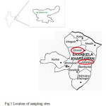Figure 1: Location of sampling sites.  Click here to View figure

 

Adityapur Industrial  (Ai) Site

Most of the smaller and middle scale companies are located in the ‘Adityapur Industrial Estate’ (33,970 acres, 53 sq. mile) which has been a Asia’s largest Industrial hub. Approximate 1,200 industries are located here and about 250 are in pipeline. There are about 20 Larger Scale Industries located like Adhunik Group, TGS, Usha Martin, RSB etc.

Agriculture (Ag) Site

Chandil is located at (22.97°N and 86.05°E). It has an average elevation of 246 metres (807 feet) and is nearly 30 kms from site AI.The natural scenery in and around Chandil is unique and enchanting. It is surrounded by agriculture land, green mountains. The Dalma mountains which are the crown of Chandil is the safe for many wild animals like Elephants, Deer, Wild Pigs, Sambhar and many species of birds and snakes. Dalma Wild Life Sanctuary (DWLS) is famous for Elephants and Deer. The main occupation of the people near this sampling site is farming, fishing, cattle rearing etc. People near to this sampling site uses wood, cow dung for burning purpose. Biomass burning of crops residue is used extensively by the habitant of this region.

Metrological Parameter

The climatic pattern is of typical tropical monsoon type with the year subdivided into three major seasons as: summer, monsoon and winter.  We fixed organized sampling in the month of April-May and December –January as shown in Fig 2. During April – May the mean maximum temperature is 35°C whereas the mean minimum temperature is 28°C and During December – January the mean maximum temperature is 22°C whereas the mean minimum temperature were 17°C. The maximum humidity, observed during the monsoon season, has mean value of 85%. The minimum mean humidity in summer (April-May) is 26 % and winter December -January is 63%. The wind speed and visibility during the sampling period was in the range of 0-6 km/h and 2-4 km respectively. The solar radiation flux during the sampling period April-May was in the range of 21.19 – 24.12 watt/m² and during the month of December-January is in range of 12.21 – 15.76 watt/m².   All meterological data are acquired from the nearest meteorological office of IMD (Indian Meteorological Department).

Sampling

Ambient 24-h integrated PM₁₀ and PM_2.5 (particulate matter less than 2.5 and 10 μm aerodynamic diameters, respectively)   samples were collected with a high volume (Hi-Vol) sampler (Thermo Scientific, MA, USA) at both site AI and AG. The sampling sites are located in urban-industrial and rural which is in the radius of 20 km from the NIT Jamshedpur, Jharkhand. Samplers were set up at ∼10-15 m above ground level at both sites. The sampling was carried in the month of April, May, Dec (2014) and Jan (2015) dated 7^th, 8^th and 9^th of above mentioned month shown in Fig 2. A total of 50 samples were collected. Pre-baked Quartz filters (8×10 in, 2500 QAT-UP; Pall Corporation, NY, USA) was used for the sampling. After sampling, the filters were swathed in aluminium foil and kept in freezer until analyses.

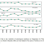Figure 2: Day to day variability of metrological conditions (a) Temperature (b) Wind Speed (WS) (c) Relative Humidity (RH) (d) Solar Radiative Flux and (e) Visibility at two Sampling Sites.  Click here to View figure

 

EC and OC Analysis

PM_1.0 and PM_2.5 Samples were analysed for EC and OC using the Thermo- Optical Transmission (TOT) method on a Sunset Lab analyser^20-21. In this method we use different temperatures to oxidised EC and OC. The chief task of the optical module of the analyzer is an alteration for the pyrolysis of organic carbon. The eight fractions OC₁, OC₂, OC₃, OC₄, EC₁, EC₂, EC₃ and PC (Pyrolyzed Carbon) are reported. The IMPROVE protocol defines OC as (OC₁ + OC₂ + OC₃ + OC₄ + PC) and EC as (EC₁ + EC₂ + EC₃ – PC). For OC analysis a filter punch is submitted to volatilization at 250, 500, 650 ⁰C for 60s  and 870°C for 90 s  in a 100% helium atmosphere, and for EC it is heated at 600, 700, 850°C for 45s and 900 ⁰C for 120s in 2% oxygen and 98% helium atmosphere. The analysis is based on liberating carbon compounds at different temperatures. At temperature 900 ⁰C the sample boat having a punch of 0.5 cm² area is passed through the oxygenator containing heated MnO₂. The concentration of CH₄ is detected by using a Flame Ionization Detector (FID) at 125°C. The initial transmittance through the filter, measured using 678 nm laser source is used to define the split-point between OC and EC and to correct for the Pyrolyzed carbon formed during initial charring of OC in a passive atmosphere. At the end of every analytical run, a fixed volume of methane (5% CH₄+95% He, Vol/Vol) is injected as an internal standard to assess the performance of FID.The overall analytical uncertainty in the measurement is calculated by summing up the absolute and relative uncertainties. Absolute uncertainty in measurement of OC (or EC) is 0.2 μg cm⁻² and TC is 0.3 μg cm⁻² while the relative uncertainty of the measured concentration is 5%.

WSOC Analysis

Before analysis one-fourth filters (̴ 105 cm² areas) was soaked Milli – Q water (7 ml for low volume filters and 20 ml for high volume filters, resistivity: 18.2 MΩ cm) and subjected to ultrasonicated for ̴ 1/2 h for extraction of the WSOC. The resulting water-extract were filtered using PTFE membrane single use syringe filters (Sartorius Minisart SRP 15) and transferred to a pre-cleaned glass vial and was analysed using a TOC liquid analyser (Shimadzu, model TC5000A). In an optimized analytical procedure, 25 ml of water – extract is injected into the furnace crammed with platinum catalyst at a temperature of 680 ⁰C, thus the CO₂ developed is measured by using a non- dispersive infrared (NDIR) detector to assess total carbon (TC) content.

Result and Discussion

Mass concentration of PM

A total of 50 PM_2.5 and PM₁₀ samples (including field blanks) was collected for this study. Mass concentration of PM₁₀ has varied from 191 to 312 µg/m³ with an averaged value of (249.1 µg/m³) at sampling site AI, minimum value during the month of May and maximum value  in the month of December Fig 3 (a). Similarly, Mass concentration of PM_2.5 has varied from 99 to 189 µg/m³ with an averaged value of (133.7 µg/m3) at sampling site AI, minimum value during the month of May and maximum value in the month of December Fig (3a).   Fig. 3 shows the variation in mass concentration of PM₁₀ and PM_2.5 of both the sampling sites. Higher concentration of PM₁₀ and PM_2.5 in the month of December-January at both the sampling sites may be due to the combined effect of source strength and lower boundary layer height²². Generally during winter, the meteorology of Jamshedpur is dominated by high pressure centered over Western Dalma hill instigating enlarged atmospheric constancy, which turn and allows less general circulation engulfing extra stagnant air masses. Moreover, deficiency of precipitation in the winter too may decrease the potential of wet deposition and allied cleansing mechanisms of the atmosphere.

PM₁₀ and PM_2.5 samples are analysed for OC, EC, and WSOC (Fig 3 b-d). It has been observed that average of total carbon (TC=OC+EC) concentration contribute ̴ 43% and ̴ 20% of PM₁₀ and PM_2.5 masses respectively, whereas, WSOC account for  ̴ 25% and  ̴ 11% of PM₁₀ and PM_2.5 masses respectively at both the sampling sites. The contribution of unidentified mass (UM), estimated by subtracting TC and WSOC concentrations from the PM₁₀ and PM_2.5 masses. The UM accounts for ̴ 32% and ̴69%, respectively, of total PM₁₀ and PM_2.5 masses. Ram and Sarin ²³have also estimated 41.4% unidentified mass of PM₁₀ at Kanpur, IGP, India whereas 42.3% and 51.5% UM of TSP at Hissar and Allahabad of IGI, India²⁴.

Spatial and temporal distributions of OC and EC

Spatial and temporal distributions of OC and EC are illustrated in Fig. 3(b, b’, c, c’). The carbon concentrations can be affected by several factors.one of such factor is Dilution and it is due to enlarged mixing depths²⁵ and particle washout on rainy days resulted in lower PM and carbon levels in the April-May. Winter time stagnation decreased the dispersion and transport of pollutants and resulted in an increase in pollution levels. OC_10, OC_2.5 concentrations at the AI and AG sites ranged from 31.7 to 53.1μg/m³, 15.3 to 28.7μg/m³ and 16.0 to 25.4 μg/m^3, 4.2 to 9.2 μg/m3, respectively Fig 3 (b, b’), whereas the corresponding EC₁₀ and EC_2.5 ranged from 6.2 to 14.6 μg/m³, 2.2 to 6.2 μg/m³ and 0.8 to 3.0 μg/m³ at sites AI and AG respectively Fig 3 (c, c’).

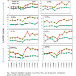Figure 3: Temporal and Spatial variability of (a) PM10, PM2.5 and the associated carbonaceous species: (b) OC (c) EC and (d) WSOC.  Click here to View figure

 

Average OC₁₀ and OC_2.5 concentrations at the AI site where nearly 2- 4 times higher than AG site Fig 3 (b, b’) and Average EC₁₀ and EC_2.5 concentrations were approx. 2-3 times higher than those at the AG site Fig 3 (c, c’). Elevated OC and EC concentrations at the AI site reflect the influence of vehicle exhaust, biomass burning, wood burning, crop residue burning along with emissions from restaurants and nearby industries. Ratios of OC to EC have been used to suggest the source of carbonaceous particles^26-27. Fig 4 shows that the, OC₁₀/EC₁₀, OC_2.5/EC_2.5,OC₁₀/PM₁₀,OC_2.5/PM_2.5,EC₁₀/ PM₁₀EC_2.5/PM_2.2  ratios at the AI and AG sampling sites varied from 2.8 – 8.3 (avg 4.9), 4.2 – 7.6 (avg 5.5), 0.17 -0.19 (avg 0.17), 0.14 – 0.20 (avg 0.17), 0.03 – 0.06 (avg 0.04), 0.02 – 0.04 (avg 0.03) and 3.3 – 8.3 (avg 4.9), 3.03 – 8.8 (avg 3.9), 0.62 – 0.98 (avg 0.78), 0.09 – 0.12 (avg 0.09), 0.07 – 0.23 (avg 0.17), 0.01 – 0.04 (avg 0.02) respectively. Whereas,²³  Ram and Sarin²³ reported the same in the range of 2.9-8.4 with an average value of 6.01±.3 at Kanpur. Low OC/PM and EC/PM ratios are primarily due to the elevated PM concentrations at the AI and AG is sampling sites, implying direct emissions from anthropogenic sources. Elevated OC/EC ratios at the local site suggested the transport of old aerosol it may have included secondary organic aerosol (SOA). However, the OC/EC ratios over Jamshedpur and some of the urban locations mentioned in the Table 1 are relatively higher than those (average :< 4.0) , Such difference in the OC /EC ratio for two dissimilar states might be due to alterations in discharge causes of carbonaceous aerosols²³.

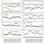Figure 4: Variation of (a) OC/PM, ( b)EC/PM, (c) WSOC/EC (d) OC/EC ratios during the sampling period at the given  study sites  Click here to View figure

 

Fig. 5 shows the scatter plot between OC₁₀ and EC₁₀ during the study period (r²=0.71; and r²=0.31) at sites AI and AG respectively. Similarly between OC_2.5 and EC_2.5 during the study period (r²=0.77; and r²=0.61) at sites AI and AG respectively. A significant correlation between OC and EC is usually revealing of their common sources like vehicular traffic¹². In contrast, a poor correlation between OC and EC specifies the formation of SOA under approving circumstances for the gas to particle alteration of VOCs through a photochemical reaction in the atmosphere. Overall, a positive linear trend is observed between OC and EC for an AI and AG sites of Jamshedpur.

WSOC Concentration

The water-soluble fraction of OC (i.e., WSOC) frequently consists of larger than 30% of PM_2.5 or PM₁₀ OC, often being related to polar compounds and correlated with SOA pattern²⁸. WSOC has the potential to modify the hygroscopic properties of particles, including PM size and cloud condensation nuclei activities²⁹. More than 80% of all WSOC were in PM_2.5 at both sites (means of 84% at AI and 82% at AG), and the ratios were relatively stable during our observation period. The PM₁₀ and PM_2.5 concentrations of WSOC at AI and AG sites ranged from 8.2 – 22.3 µg/m³ (avg 15.68 µg/m³), 4.3 – 8.4 µg/m³ (avg 6.8 µg/m³), 3.4 – 7.9 µg/m³ (avg 5.8), 2.1 -5.3 µg/m³ (avg 4.1) respectively Fig 3(d,d’). The concentrations of WSOC₁₀ and WSOC_2.5 were higher in December and January and low in the month of April and May.

Fig. 5 shows the relationships between WSOC₁₀ and WSOC_2.5 with (a) OC₁₀ and OC_2.5, (b) PM₁₀ and PM_2.5, and (c) EC₁₀ and EC_2.5 at AI and AG sites. The regression lines between WSOC₁₀ (r²-0.82) and PM₁₀ (r²-0.6) were almost the same for WSOC_2.5 (r²-0.82 and EC_2.5 (r²-0.64) at AI and AG respectively. The regression lines for WSOC₁₀ and OC₁₀, and WSOC_2.5 and OC_2.5 however, were quite different. We also examined the WSOC₁₀/OC₁₀, WSOC_2.5/OC_2.5, WSOC₁₀/EC₁₀; WSOC_2.5/EC_2.5 ratio in Fig. 4 for AI and AG sampling sites. The WSOC/OC and WSOC/EC ratios for PM₁₀ and PM_2.5 ratios at site AI ranged from 0.24 to 0.45 µg/m³ (avg 0.35 µg/m³), 1.30 to1.85 µg/m³ (avg 1.51 µg/m³), 0.18 to 0.29 µg/m³ (avg 0.25 µg/m³), 1.34 to 1.83 µg/m³ (avg 1.4 µg/m³) respectively. Again for the site AG the WSOC/OC and WSOC/EC ratios for PM₁₀ and PM_2.5 ratios ranged from 0.25 to 0.44 µg/m³ (avg 0.33 µg/m³), 1.34 to 2.24 µg/m³ (avg 1.60 µg/m³), 0.30 to 0.68 µg/m³ (avg 0.54 µg/m³), 1.62 to 3.50 µg/m³ (avg 2.06 µg/m³) respectively Fig (4).  The ratios did not vary considerably by season, but they did tend to increase slightly in April and May and decrease in December and January. Ambade¹ accounted WSOC/OC ratios of 0.61 in August, 0.64 in June, and 0.31 in October at an urban site, and WSOC/OC ratios boost under high photochemical vigorous state. Miyazaki³⁰ quoted WSOC/OC ratios of 0.35 in summer and 0.19 in winter 2004 in Tokyo. In this study, the WSOC/OC ratio also increased in April-May, when photochemical reactions are most active.

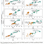Figure 5: Correlation between  (a) OC and EC (b) WSOC and OC (c) WSOC and PM (d) WSOC and EC  for the two sampling sites.  Click here to View figure

 

The WSOC/EC ratios for PM₁₀ and PM_2.5 were much higher on AG site. The average WSOC/EC ratio PM₁₀ and PM_2.5 1.60 and 2.06. The difference in the WSOC/EC and WSOC/OC ratios between sites AG and AI indicates that the chemical components and EC characteristics were different; the higher WSOC/EC ratio suggested that the EC at was more oxidized in the atmosphere. This disparity between the two sites could be caused by disparities in primary emissions and secondary formation among the sites. Primary EC is predominantly water-insoluble³⁰, and there are primary EC sources (e.g., vehicles) in site AI, whereas there are very few sources of primary EC at site AG. Conversely, secondary formation is probably promoted during the transport of pollutants to site AG. Therefore, the WSOC ratios fraction at site AG was higher than that at site AI.

Comparison of OC and EC with other Asian cities

Table 1 compares WSOC, OC, and EC concentrations in PM_2.5 and PM₁₀ from 11 cities across the world. EC₁₀ concentration of study site AI ranked the highest. The concentration of WSOC, EC, and OC at Kanpur²³ is 2-5 times more than present study sites; this may be due to more motor vehicles and more coal use at the Kanpur.   While OC_2.5 concentrations at site AG were similar toBeijing (China)³¹ and for AI site the concentration of OC_2.5 is nearly 2-5,3-5,1.5,1.5,4.5,1.5,1.5 times than Hong Kong³², Thessaloniki (Greece)³³, PRDR(China)³⁴, Shanghai (China)³¹, Lanzhou(China), Guangzhou(China)³¹, respectively. EC_2.5 concentrations at site AI were similar in Hong Kong³², Thessaloniki (Greece)³³, Beijing (China)31. WSOC_2.5 show similar behavior in Shanghai (China)³¹ at site AI and for site AG it is similar to Beijing (China)³¹.

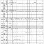Table 1: Comparative study of present study with worldwide. Click here to View table

 

Summary and Conclusion

The present study has demonstrated spatial and temporal variations in concentration of OC, EC, and WSOC in (PM₁₀ +PM_2.5) level at two inland locations on the Jamshedpur during April- May 2014 and January 2104 – December 2015 respectively.

• Average OC₁₀ and OC_2.5 concentrations during the sampling period were 43.2 μgm⁻³ and 22.6 μg/m³ at site AT and 20.3 μg/m³ and 7.7 μg/m³at site AG, respectively; EC concentrations were 10.4 μg/m³, 4.2 μg/m³ and 4.4 μg/m³, 2.1 μg/m³, respectively; This indicates that carbonaceous aerosol is the dominant component in the AI sampling site.
• All of the (PM₁₀ and PM_2.5) OC/EC ratios exceeded 4.0, and average OC/EC ratios were 4.3 and 5.5 at site AI and 4.9 and 3.9 at AG site. Elevated OC/EC ratios were found during heating seasons with increased primary emissions, such as residential coal combustion, nearby vehicle emissions. OC/EC ratios were higher owing to the formation of SOA during transport.
• (PM₁₀ and PM_2.5) WSOC concentrations were 15.68 μg/m³, 5.8 μg/m³ and 6.8 μg/m³, 4.1 μg/m³ at AI and AG sampling sites respectively. WSOC between an AT/AG pair indicated that on average AT WSOC was 49% higher than AG levels during the sampling period. The AT excess WSOC was clearly associated with local anthropogenic emissions since the WSOC enhancement was linked to CO and NOx. We also inferred that WSOC was produced by photochemical reaction and was caused by the combustion of both fuel and biomass.

References

1. Ambade, B. Lap-Lambert Academic Publishing, Germany. 2012, ISBN: 978-3-659-30271-8.
2. Malm, W.C.; Day, D.E. Atmos. Environ. 2000, 34, 3373–3391.
   CrossRef
3. Dreher, K.L. Inhalation Tox. 2000, 12 (supp 3), 45–57.
   CrossRef
4. IPCC. Cambridge Univ. Press. New York, 2007.
5. Castro, L.M.; Pio, C.A,; Harrison, R.M.; Smith, D.J.T. Atmos. Environ.1999, 33, 2771–2781.
   CrossRef
6. Andrews, E.; Saxena, P.; Musarra, S.; Hildemann, L.M.; Koutrakis, P.; McMurry, P.H.; Olmez, I.; White, W.H. J. Air Waste Manage. Assoc. 2000, 50, 648– 664.
   CrossRef
7. Ambade, B.; Ghosh, S. Nat. Hazard. 2013, 69, 589–598.
   CrossRef
8. Bond, T.C.; Street, D.G.; Yarber, K.F.; Nelson, S.M.; Woo, J.H.; Klimont, Z. J. Geophys. Res. 2004, 109, D14203.
   CrossRef
9. Wonaschutz, A.; Hersey, SP.; Sorooshian, A.; Craven, J.S.; Metcalf, A.R.; Flagan, R.C.; Seinfeld, JH. Atmos. Chem. Phys. 2011, 11, 8257-8270.
   CrossRef
10. Streets, D.G.; Yarber, K.F.; Woo, J.H.; Carmichael, G.R. Glob. Biogeochem. Cycles. 2003, 17.
11. Seinfeld, J.H.; Pandis, S.N. Wiley., New York. 1998
12. Salma, I.; Chi, X.; Maenhaut, W. Atmos. Environ. 2004, 38, 27–36.
    CrossRef
13. Hu, W.W.; Hu, M.; Deng, Z.Q.; Xiao, R.; Kondo, Y.; Takegawa, N. Atmos. Chem. Phys. 2012, 12, 1811–22.
    CrossRef
14. Ambade, B. Urban Climate. 2014, 9, 155-165.
    CrossRef
15. Feng, Y.; Chen, Y.; Guo, H.; Zhi, G.; Xiong, S.; Li, J.; Sheng, G.; Fu, J. Atmos. Res. 2009, 92, 434–442.
    CrossRef
16. Vutukuru, S.; Griffin, R.J.; Dabdub, D. J. Geophys. Res. 2006, 111, D10S12.
    CrossRef
17. Nieuwenhuijsen, M.J.; Dadvand, P.; Grellier, J.; Martine, D.; Vrijheid, M. Environ. Health. 2013, 12, 6.
    CrossRef
18. Eisner, M.D. Thorax. 2010, 65, 229-234.
    CrossRef
19. Brook, R.D.; Rajagopalan, S.; Pope, C.AIII.; Brook, J.R.; Bhatnagar, A.; Diez-Roux, A.V. Circulation. 2010, 121, 2331–2378.
    CrossRef
20. Ram, K.; Sarin, M.M.; Hegde, P. Atmos. Environ. 2008, 42, 6785–6796
    CrossRef
21. Rengarajan, R.; Sarin, M.M.; Sudheer, A.K. J. Geophys. Res. 2007, 112, D21307.
    CrossRef
22. Datta, A.; Saud, T.; Goel, A.; Tiwari, S.; Sharma, S.K.; Saxena, M.; Mandal, T.K. J. Atmos. Chem. 2010, 65, 127–143.
    CrossRef
23. Ram, K.; Sarin, M.M. Atmos. Environ. 2011, 45, 460–468.
    CrossRef
24. Ram, K, Sarin, M.M., Sudheer, A.K.; Rengarajan, R. Aeros. Air Qual. Res. 2012, 12, 359–370.
    CrossRef
25. Sequeira, R.; Lai, K.H. Atmos. Environ. 1998, 32, 133–144.
    CrossRef
26. Turpin, B.J.; Huntzicker, J.J. Atmos. Environ. 1995, 29, 3257–3544.
    CrossRef
27. Chow, J.C.; Watson, J.G.; Lowenthal, D.H.; Solomon, P.A.; Magliano, K.L.; Ziman, S.D.; Richards, L.W. Aerosol Sci. Technol. 1993, 18, 105–128.
    CrossRef
28. Rogge, W.F.; Mazurek, M.A.; Hildemann, L.M.; Cass, G.R.; Simoneit, B.R.T. Atmos. Environ. 1993, 27A, 1309–1330.
    CrossRef
29. Shulman, M.L.; Jacobson, M.C.; Charlson, R.J.; Synovec, R. E.; Young, T.E. Geophys. Res. Lett. 1996, 23, 277–280.
    CrossRef
30. Miyazaki, Y.; Kondo, Y.; Takegawa, N.; Komazaki, Y.; Fukuda, M.; Kawamura. J. Geophys. Res. 2006, 111.
31. Pathak, R.K.; Wang, T.; Ho, K.F.; Lee, .SC. Atmos. Environ. 2010, 45, 318 – 325.
    CrossRef
32. Ho, K.F.; Lee, S.C.; Cao, J.J.; Li, Y.S.; Chow, J.C.; Watson, J.G.; Funk, K. Atmos. Chem. Phys. 2006, 6, 4569-4576.
    CrossRef
33. Samara, C.; Voutsa, D.; Kouras, A.; Eleftheriadis, K.; Maggos, T.; Saraga, D.; Petrakakis, M. Environ. Sci. Pollut. Res. 2013, 21, 1769–1785.
    CrossRef
34. Cao, J.J.; Lee, S.C.; Ho, K.F.; Zhang, X.Y.; Zou, S.C.; Fung, Kochy.; Chow, C.J.; Watson, J.G. Atoms. Environ. 2003, 37, 1451-1460.
    CrossRef

---

This work is licensed under a Creative Commons Attribution 4.0 International License.